Quantum Dynamics Simulations of the 2D Spectroscopy for Exciton Polaritons

From the paper

How do phonons and cavity loss shape polariton spectra?

Strong coupling between a molecular excitation and a confined photon creates upper and lower polaritons. Their optical response is governed by two distinct environments: molecular vibrations perturb the excitonic component, while photon leakage removes the cavity component. Linear absorption can show the polariton splitting and linewidths, but it does not cleanly separate frequency memory, coherent energy exchange, and the individual nonlinear response pathways.

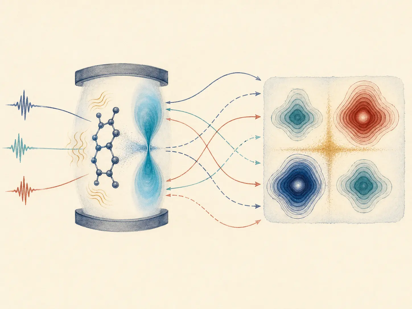
The paper develops a trajectory approach for calculating both linear spectra and two-dimensional electronic spectra while retaining an explicit, non-Markovian phonon bath and a lossy cavity. It then asks how increasing the light-matter coupling $g_c$ or cavity loss rate $\Gamma$ changes polariton linewidths, cross peaks, and coherence lifetimes.

From the paper

A molecular exciton, an explicit phonon bath, and one lossy cavity mode

For localized exciton states $|m\rangle$, the molecular Hamiltonian is

Here $\bar\epsilon$ is a reference excitation energy, $\epsilon_m$ is a site-energy offset, and $J_{mn}$ couples localized excitons. Each site has an independent harmonic environment,

The frequencies and couplings represent a Debye spectral density,

where $\lambda$ is the reorganization energy and $\omega_0$ is the bath cutoff frequency. The cavity and rotating-wave light-matter interaction are

The transition dipoles are taken parallel to the cavity polarization and permanent dipoles are neglected. The calculation includes the ground, single-excitation, and relevant double-excitation sectors so that excited-state absorption can be evaluated.

Elementary origin of polaron decoupling

For one resonant molecule, the two bright eigenstates are

Only the molecular component couples directly to the phonons. Consequently,

which is half the diagonal coupling of the bare molecular excitation in this simple resonant example. This reduced vibrational displacement is the elementary polaron-decoupling argument used to interpret the narrower polariton lines and longer coherence.

From the paper

L-PLDM combines non-Markovian phonons with stochastic cavity loss

The partial linearized density matrix method represents each reduced-density-matrix contribution with separate forward and backward electronic-photonic amplitudes. The bath coordinates follow a mean force constructed from both paths. Because the phonons are propagated explicitly rather than replaced by a memoryless rate, their feedback on the quantum subsystem is retained within the PLDM approximation.

Cavity leakage is represented by a Lindblad dissipator,

In L-PLDM, complex random factors update the forward and backward mapping amplitudes. Their ensemble average reproduces the Lindblad population transfer and coherence damping. The full time step uses a symmetric split:

1. FocusSample the dipole-created density-matrix element and initialize forward and backward amplitudes.
2. PropagateEvolve the amplitudes and explicit bath, with half-step stochastic loss on either side.
3. AverageCombine weighted trajectories and Fourier transform the response into a spectrum.

For 2DES, this procedure is repeated after each laser interaction. Importance sampling selects one density-matrix branch according to its magnitude and carries its complex phase as a trajectory weight, preventing an explicit expansion over every possible branch.

From the paper + visual guide

From four dipole interactions to diagonal and cross peaks

The third-order response can be written as a nested commutator,

The commutator expands into rephasing and non-rephasing pathways. Each group contains ground-state bleaching (GSB), stimulated emission (SE), and excited-state absorption (ESA). Fourier transforming $t_1$ and $t_3$, then adding the rephasing and non-rephasing signals, gives the purely absorptive spectrum.

• Diagonal peaks: excitation and detection occur at the same lower- or upper-polariton frequency.
• Cross peaks: excitation at one polariton frequency is correlated with detection at the other; their $t_2$-dependent oscillation reports upper-lower coherence.
• ESA features: transitions from the single- to double-excitation manifold can be shifted along the detection axis because the two excitation gaps are unequal.
• Lineshape: cavity loss adds homogeneous, anti-diagonal broadening, while slow frequency fluctuations preferentially elongate a diagonal peak along the diagonal.

Simplified educational example

A lossy two-state polariton explains splitting contraction

Ignore the explicit phonon coordinates for a moment and replace their bare molecular broadening by $\gamma$. In the basis $\{|e,0\rangle,|G,1\rangle\}$, use the effective non-Hermitian Hamiltonian

At resonance, $E_e=E_c=E_0$, its complex poles are

import numpy as np
import matplotlib.pyplot as plt

G = 456.0       # light-matter coupling energy, cm^-1
gamma = 175.0   # bare molecular linewidth parameter, cm^-1
omega = np.linspace(-1200.0, 1200.0, 2401)

def polariton_spectrum(Gamma):
    H_eff = np.array([
        [-0.5j * gamma, G],
        [G, -0.5j * Gamma],
    ], dtype=complex)
    poles = np.linalg.eigvals(H_eff)
    signal = np.zeros_like(omega)
    for pole in poles:
        width = max(-pole.imag, 1.0)
        signal += width / ((omega - pole.real)**2 + width**2)
    return poles, signal / signal.max()

for Gamma in (0.0, 400.0, 800.0):
    poles, signal = polariton_spectrum(Gamma)
    print(f"Gamma={Gamma:5.1f} cm^-1, poles={poles}")
    plt.plot(omega, signal, label=fr"$\Gamma={Gamma:.0f}$ cm$^{{-1}}$")

plt.xlabel(r"Frequency relative to resonance (cm$^{-1}$)")
plt.ylabel("Normalized illustrative absorption")
plt.legend()
plt.tight_layout()
plt.show()

From the paper

What the simulations report

• Linear-spectrum validation: for the resonant monomer, the simulated loss-dependent polariton positions and broadening closely follow the analytic lossy Jaynes-Cummings model.
• Polaron-decoupled linewidths: in a lossless cavity, the calculated polariton peaks are narrower than the bare molecular absorption line because the photonic component does not couple directly to the phonon bath.
• Competing role of cavity loss: increasing $\Gamma$ broadens the peaks, contracts the splitting, and eventually merges the polariton doublet. In 2DES it adds homogeneous broadening and accelerates signal decay.
• Cross-peak dynamics: larger $g_c$ separates the polariton peaks and produces more prominent upper-lower cross-peak oscillations.
• Bright and dark dimer states: the chosen asymmetric dimer has upper, lower, and middle polaritons. The middle state is effectively dark because its ground-state transition dipole is about 35 times smaller than those of the bright polaritons.
• Pathway balance: GSB and SE dominate the reported dimer spectra; ESA is weaker for the selected parameters, although its shifted transitions explain derivative-like structure.
• Longer model coherence: at 300 K, stronger coupling yields polaritonic oscillations persisting beyond 200 fs, compared with bare electronic coherence that decays in less than about 50 fs for the chosen dimer and bath. Long-lived oscillations remain for $\Gamma=10$ meV and a Rabi splitting near 124 meV.

Scope and limitations

What should not be generalized without further tests

• The demonstrations use a monomer and one asymmetric dimer, not a macroscopic collective ensemble.
• The light-matter model contains one cavity mode and uses the rotating-wave approximation; counter-rotating and dipole self-energy terms are absent.
• The molecular phonons are explicitly non-Markovian, but photon leakage is treated as a Markovian Lindblad process.
• PLDM is a semiclassical, partially linearized approximation rather than an exact solver for arbitrary system-bath parameters.
• The phonon environment is a finite discretization of a Debye spectral density, so linewidths and coherence lifetimes depend on the selected $\lambda$, $\omega_0$, temperature, and discretization.
• The dipoles are assumed aligned with the cavity field, permanent dipoles are neglected, and static energetic or orientational disorder is not included in these model calculations.
• The reported coherence enhancement is a result for the stated model and parameters. It is not a universal lifetime prediction for every molecular cavity.
• The code example above explains only the lossy two-state poles and should not be compared quantitatively with the full L-PLDM 2DES.