Polariton spectra under the collective coupling regime. II. 2D non-linear spectra

From the paper

How can collective-coupling 2DES avoid the density-matrix bottleneck?

Two-dimensional electronic spectroscopy resolves excitation and detection frequencies independently. It can separate homogeneous and inhomogeneous broadening, reveal upper-lower polariton coherences through cross peaks, and expose excited-state absorption (ESA) into the double-excitation manifold. Those capabilities make 2DES a sensitive test of collective polaron decoupling, but they also make a direct calculation expensive.

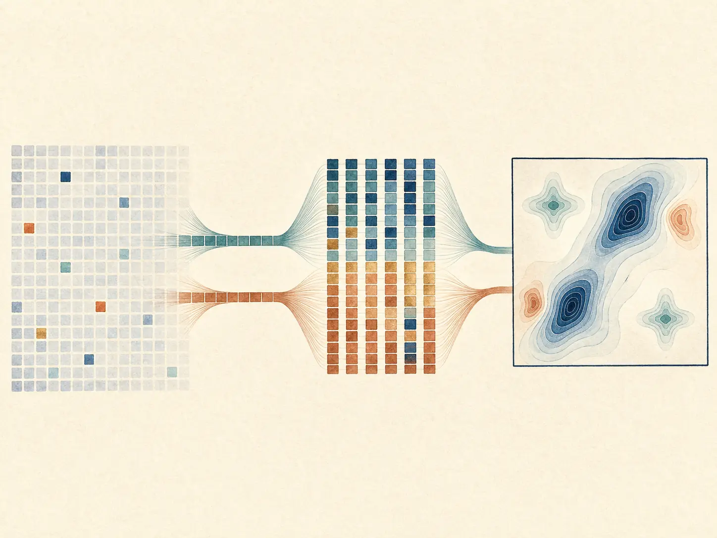
For $N$ molecules, the double-excitation Hilbert space already grows quadratically. An explicit density matrix then contains the square of that number of amplitudes, while a conventional three-delay workflow branches across $t_1$, $t_2$, and $t_3$. The paper asks whether sparse state-vector propagation, a forward-backward factorization, and vectorized batching can retain the required nonlinear pathways without constructing the full density matrix.

1. Keep state vectorsPropagate one forward ket and one backward bra instead of a dense reduced density matrix.
2. Sample two indicesFactor a two-dimensional importance distribution into two one-dimensional distributions.
3. Batch the delaysAdvance trajectories and delay branches together, within the available GPU memory.

From the paper

The HTC model must include two excitation manifolds

The quantum subsystem contains $N$ two-level molecular excitons, one cavity mode, and diagonal coupling to an independent harmonic bath for each molecule. Under the rotating-wave approximation,

The dipole operator $\hat\mu=\sum_n\mu_n(\hat\sigma_n^\dagger+\hat\sigma_n)$ moves the system among the ground, single-excitation, and double-excitation sectors. The latter is essential for ESA. The total basis size used in the paper is

The terms represent localized single excitons, photon-dressed states, molecular excitation pairs, molecule-plus-photon states, and the two-photon state. For example, the stated expression gives $K=5$, $8$, and $23$ for $N=1$, $2$, and $5$. An explicit $K\times K$ density matrix therefore scales as $O(N^4)$ in storage, and a dense density-matrix action can reach $O(N^6)$ work. The sparse formulation instead stores $O(N^2)$ state vectors and applies only physically connected Hamiltonian and dipole operations.

The exciton-phonon dynamics are approximated with partially linearized density-matrix (PLDM) trajectories. Photon leakage can be included through stochastic Lindblad dynamics; together the framework is called L-PLDM.

From the paper

A mixed density matrix from forward and backward state vectors

Each trajectory carries a forward state $|\psi\rangle$ and an independently evolving backward state $|\widetilde\psi\rangle$. Their coefficients satisfy conjugate Schrödinger equations while the classical bath evolves under the mean of the two path forces. A trajectory contributes the rank-one estimator

The method never needs to materialize that outer product. After a dipole acts on the forward path, define $|\phi\rangle=\hat\mu|\psi\rangle$. The response contribution is the overlap

This is the central computational change: the same mixed-state information is recovered statistically from rank-one forward-backward estimators and scalar overlaps rather than by propagating all $K^2$ matrix elements.

From the paper

Factorized importance sampling replaces a $K^2$ search

A laser interaction can create many possible density-matrix elements. Write the amplitudes after the dipole action as

The magnitude of outer-product element $(a,b)$ is $r_a\widetilde r_b$. Its normalization factor separates exactly:

One can therefore sample $a$ from $p_a=r_a/\sum_jr_j$ and $b$ from $q_b=\widetilde r_b/\sum_j\widetilde r_j$. The complex phase $e^{i(\varphi_a-\widetilde\varphi_b)}$ is retained in the trajectory weight. Building and searching two cumulative distributions costs $O(2K)$, rather than constructing a $K\times K$ probability table.

import numpy as np

rng = np.random.default_rng(7)
phi = np.array([1.0, 0.5j, -0.25])
psi_tilde = np.array([0.5, -1.0j])

p = np.abs(phi) / np.abs(phi).sum()
q = np.abs(psi_tilde) / np.abs(psi_tilde).sum()
target = np.outer(p, q)

counts = np.zeros_like(target)
for _ in range(100_000):
    a = rng.choice(len(p), p=p)
    b = rng.choice(len(q), p=q)
    counts[a, b] += 1

sampled = counts / counts.sum()
print("explicit probabilities:\n", target)
print("sampled probabilities:\n", sampled)

From the paper

GPU batching trades memory for delay-grid time

Independent trajectories and states created at different delay points can be stored as columns of a batch matrix. Sparse HTC operations then act on many columns simultaneously through vectorized elementwise products and reductions. The paper describes a hierarchy of batching choices:

1. One delay batchedIdeal delay-grid work changes from $O(T^3)$ to $O(T^2)$.
2. Two delays batchedThe ideal time dependence falls to $O(T)$, with a larger resident batch.
3. Three delays batchedIdeal operation time approaches $O(T^0)$ only when memory can hold the full delay cube.

The final line is a runtime idealization, not a claim that the data volume disappears. A $T^3$ set of response points still exists, and full batching can require substantial GPU memory. Practical calculations choose how many of $t_1$, $t_2$, and $t_3$ to vectorize according to the available accelerator memory.

Simplified educational example

Build a four-peak absorptive spectrum from analytic teaching shapes

Place lower and upper polariton frequencies at $-50$ and $+50$ meV relative to resonance. Positive ground-state-bleach (GSB) peaks occupy all four LP/UP coordinates. Rephasing stimulated emission (SE) can reinforce diagonal and cross peaks, while a simple nonrephasing bright-state SE path contributes only diagonal peaks. Negative ESA features are displaced by $+8$ meV along the detection-frequency direction because the ground-to-single and single-to-double gaps are unequal.

Reducing the Gaussian widths can mimic the collective narrowing reported as $N$ increases. Damping the SE amplitude more rapidly than GSB during $t_2$ gives a qualitative picture of how cavity loss reweights the pathways. These controls are explanatory analogies only; a production spectrum requires the full forward-backward trajectory average and Fourier transforms over $t_1$ and $t_3$.

import numpy as np
import matplotlib.pyplot as plt

w = np.linspace(-120.0, 120.0, 401)  # meV relative to resonance
w1, w3 = np.meshgrid(w, w, indexing="xy")

def peak(x0, y0, sigma_diag=26.0, sigma_anti=10.0):
    u = ((w1-x0) + (w3-y0)) / np.sqrt(2.0)
    v = ((w1-x0) - (w3-y0)) / np.sqrt(2.0)
    return np.exp(-0.5*((u/sigma_diag)**2 + (v/sigma_anti)**2))

bright = (-50.0, 50.0)
gsb = sum(peak(x, y) for x in bright for y in bright)
se = sum(peak(x, y) for x in bright for y in bright)
esa = -0.45*sum(peak(x, y+8.0) for x in bright for y in bright)
absorptive = gsb + se + esa

plt.contourf(w1, w3, absorptive, levels=31, cmap="RdBu_r")
plt.xlabel(r"$\hbar\omega_1$ relative to resonance (meV)")
plt.ylabel(r"$\hbar\omega_3$ relative to resonance (meV)")
plt.colorbar(label="toy response")
plt.show()

From the paper

What the collective calculations report

• Density-matrix avoidance: sparse forward-backward state vectors reduce the formal double-manifold propagation from an $O(N^6)$ dense density-matrix problem to $O(N^2)$ state-vector storage and sparse actions.
• Collective narrowing: rephasing, nonrephasing, and absorptive spectra for $N=1,2,5,25$ become progressively narrower at fixed collective Rabi splitting, consistent with reduced effective vibrational reorganization.
• Changing pathway balance: the relative nonrephasing contribution grows with $N$, and the total lineshape becomes more homogeneous as coupling to slow bath fluctuations is reduced.
• Collective ESA structure: for $N>1$, unequal spacings in the single- and double-excitation ladders shift negative ESA lobes and create derivative-like polariton features.
• Dark states remain optically silent: they do not appear directly in the symmetric spectra because their collective transition dipole cancels.
• Finite-$t_2$ loss: in the $N=5$ pathway study, SE cross peaks weaken as photonic population leaks during $t_2$, whereas GSB remains in the ground-state population and becomes the dominant later-time rephasing cross-peak contribution.
• Coherent beating: upper-lower coherence pathways make cross-peak intensity oscillate at the Rabi splitting.

Scope and source cautions

What the scaling claims do and do not mean

• The largest reported collective 2DES spectrum contains $N=25$ molecules. This is much smaller than the ensembles reached for linear spectra because the nonlinear calculation must retain the double-excitation sector.
• The $N$-dependence series is evaluated at $t_2=0$ without cavity loss. The finite-$t_2$ pathway decomposition instead uses $N=5$ and $\Gamma_c=10$ meV.
• The displayed spectra use one cavity mode, two-level molecules, the rotating-wave approximation, independent discretized Debye baths, and no explicit static energetic or orientational disorder.
• L-PLDM is a trajectory approximation for nonadiabatic exciton-phonon dynamics, not an exact reduced-density-matrix solver.
• The ideal $O(T^0)$ timing requires full delay batching and sufficient GPU memory. It does not make response storage independent of $T$, and partial batching restores $O(T)$ or $O(T^2)$ work.
• The reported primitive timing test should not be described as an end-to-end wall-time benchmark for a complete 2DES calculation.
• Each $N$-comparison spectrum is normalized independently, so the figures establish lineshape and relative pathway trends rather than absolute oscillator-strength scaling.
• The reference excitation energy is shifted to 0.5 eV for numerical efficiency; relative frequencies and lineshapes carry the intended physical information.

This tutorial's Gaussian heatmap and sampling script are pedagogical additions. They explain the algebra and spectral reading but do not reproduce the paper's L-PLDM trajectories, GPU implementation, or reported spectra.