Polariton Spectra under the Collective Coupling Regime. I. Efficient Simulation of Linear Spectra and Quantum Dynamics

From the paper

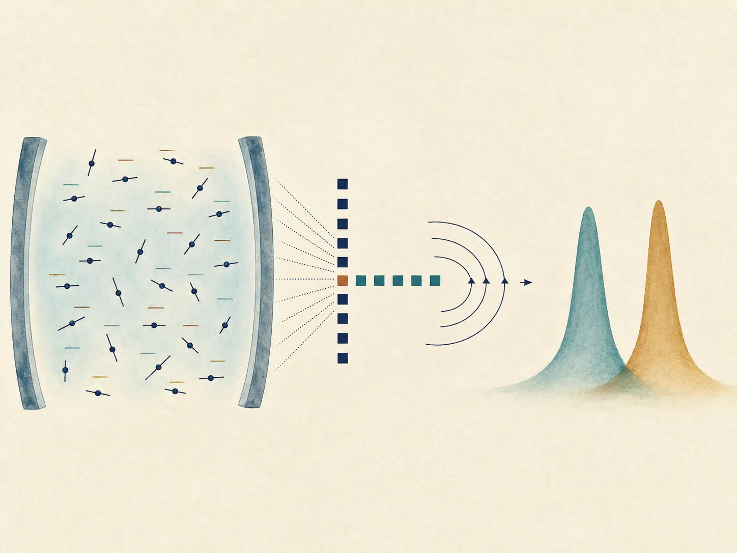
How can molecule-resolved polariton dynamics reach collective experimental sizes?

Collective strong-coupling experiments may involve thousands to millions of emitters. Static energy disorder, dipole-orientation disorder, and independent phonon fluctuations make those emitters inequivalent, so one cannot rely only on a perfectly symmetric bright-state reduction. The paper instead asks which matrix elements are physically connected and evaluates only those connections. This preserves molecule-resolved disorder while making the cost proportional to the state-vector size rather than the square of that size.

From the paper

Holstein-Tavis-Cummings model with local environments

The system contains $N$ uncoupled two-level molecular excitons and one cavity mode under the rotating-wave approximation. Every molecule has an independent harmonic bath with a Debye spectral density. Site energies may carry Gaussian static disorder, while in-plane angular disorder changes both the cavity coupling and laser coupling through the projected transition dipole. The collective Rabi splitting is held fixed as $N$ changes, so an identical single-molecule coupling would scale as $g_c\propto N^{-1/2}$.

From the paper

The single-excitation Hamiltonian is an arrowhead, not a dense network

In the ordered basis $\{|e_1,0\rangle,\ldots,|e_N,0\rangle,|G,1\rangle\}$, molecules do not couple directly to one another. Each exciton connects only to itself and to the common photon:

For $|\psi\rangle=(c_1,\ldots,c_N,c_c)^T$, one can apply this matrix without constructing it:

The dense array has $(N+1)^2$ slots, but the arrowhead has only $3N+1$ nonzero entries. The paper generalizes the same idea through the double-excitation sector: the number of basis states then grows as $O(N^2)$, yet the Hamiltonian action remains linear in that basis size rather than quadratic.

From the paper

Shift first, then propagate with a Chebyshev recurrence

A Chebyshev expansion is stable only after the Hamiltonian spectrum is mapped to $[-1,1]$. With estimated bounds $\epsilon_{\min}$ and $\epsilon_{\max}$, define $\Delta E=\epsilon_{\max}-\epsilon_{\min}$ and

The propagated state is a Bessel-weighted sum of these recurrence vectors. A second improvement removes the large common optical energy from each excitation manifold. The known phase associated with $\nu\bar\epsilon$ is restored analytically, while Chebyshev propagation acts only on the much narrower fluctuation Hamiltonian $\Delta\hat H^{(\nu)}$. This substantially lowers the required expansion order.

1. ShiftRemove the common eV-scale optical phase from each excitation manifold.
2. RescaleMap the remaining fluctuation spectrum into the Chebyshev interval.
3. RecurApply only sparse Hamiltonian-vector operations until the Bessel terms converge.

From the paper

From sparse propagation to a linear absorption spectrum

The shifted Chebyshev step is embedded in Lindblad-partially linearized density matrix dynamics. Forward and backward quantum amplitudes evolve alongside classical bath coordinates; stochastic Lindblad steps represent cavity leakage. The dipole operator is also applied as a sparse vector action, and focused sampling avoids explicitly launching every equivalent initial molecular coherence.

The reported calculation uses a cosine apodization $W(t)$ before Fourier transformation. Only the ground and single-excitation sectors are required for this linear response; the double-excitation sparse algebra is developed as groundwork for nonlinear spectroscopy.

Simplified educational example

Four molecules: dense matrix and sparse action give the same vector

import numpy as np

N = 4
epsilon = 2.0 + np.array([-0.04, -0.01, 0.02, 0.05])  # eV
omega_c = 2.0
Omega_R = 0.2
g = np.full(N, Omega_R / (2.0 * np.sqrt(N)))

rng = np.random.default_rng(7)
psi = rng.normal(size=N + 1) + 1j * rng.normal(size=N + 1)
psi /= np.linalg.norm(psi)

def arrowhead_action(vector):
    out = np.empty_like(vector)
    out[:N] = epsilon * vector[:N] + g * vector[N]
    out[N] = omega_c * vector[N] + np.dot(g, vector[:N])
    return out

# Dense reference is appropriate only for this small validation.
H = np.diag(np.r_[epsilon, omega_c]).astype(complex)
H[:N, N] = g
H[N, :N] = g

error = np.max(np.abs(arrowhead_action(psi) - H @ psi))
print("nonzero entries:", np.count_nonzero(H), "of", H.size)
print("maximum action error:", error)

The next educational step is to wrap arrowhead_action in the normalized three-term Chebyshev recurrence and compare one short propagation step with scipy.linalg.expm. That test validates the tutorial implementation; it does not reproduce the paper's L-PLDM bath ensemble.

From the paper

What the simulations report

• At fixed collective splitting, increasing $N$ lengthens the response coherence and narrows the polariton lines through collective polaron decoupling.
• The no-static-disorder convergence study directly reaches $N=10^5$; for the selected parameters, a much smaller ensemble is already visually close to that large-$N$ lower-polariton line.
• Independent energetic disorder broadens and lowers the polariton peaks. At sufficiently strong disorder, the LP and UP begin to merge.
• In-plane orientational disorder mainly contracts the Rabi splitting as the projected couplings average down, with substantially less extra linewidth broadening than energetic disorder.
• Against exact small-system propagation, the shifted Chebyshev scheme is the most accurate of the tested practical integrators over the relevant time steps.

Scope and limitations

Where the efficiency claim applies

• The physical model uses one cavity mode, two-level molecules, the rotating-wave approximation, independent Debye baths, and no direct intermolecular excitonic coupling.
• L-PLDM treats the explicit phonon dynamics approximately, and cavity loss is represented through a Markovian stochastic Lindblad model.
• The $N=10^5$ demonstration is the no-static-disorder convergence case; the broken-symmetry energy- and orientation-disorder examples use $N=500$.
• The orientation distribution is modeled in a two-dimensional plane, not as an arbitrary three-dimensional molecular distribution.
• Linear spectra use only the single-excitation sector. Double-excitation scaling should not be presented as part of the linear observable itself.
• $O(K)$ Hamiltonian actions describe ideal arithmetic scaling; trajectory count, bath propagation, memory movement, spectral-bound estimation, and hardware overhead still affect total runtime.
• The manifold energy shift preserves relative line shapes but the removed absolute optical frequency must be restored when reporting a physical spectrum.