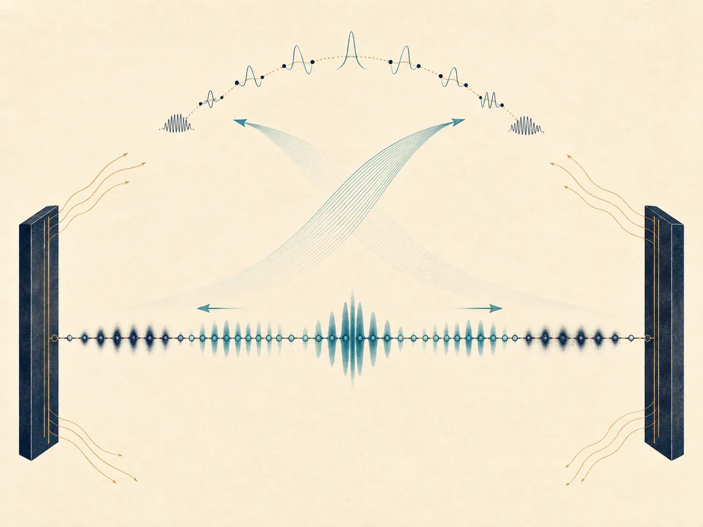
From the paper
Simulating transport at the spatial scale of experiments
Experiments image polariton motion over micrometers, yet measured wavefront velocities are often below the derivative of the ideal lower-polariton dispersion. The calculation must include thousands of molecular sites, hundreds of dispersive photon modes, local phonon environments, and photon loss. The paper develops a method that retains this spatial structure without storing the dense exciton–photon coupling matrix.
From the paper
Generalized HTC Hamiltonian
The finite-$k$ phase factors couple a real-space molecular array to a photon momentum grid. Each exciton has a classical Debye bath propagated with mean-field Ehrenfest forces, and every cavity mode undergoes phenomenological Lindblad loss. Phase-matched bright excitons form momentum-resolved upper and lower polaritons; molecular Fourier components without a matching photon remain dark.
From the paper
Why the FFT changes the feasible system size
The exciton–photon block is a discrete Fourier transform. Applying it with FFTs changes the dominant action from a dense quadratic operation to approximately $O(N\log N)$. The production workflow then:
- Build the dispersive photon grid and uniformly spaced molecular array.
- Prepare a localized polariton wavepacket from an energy-selected band.
- Sample independent molecular baths from a thermal Wigner distribution.
- Propagate quantum amplitudes with RK4 and the FFT Hamiltonian action.
- Advance classical bath coordinates with velocity Verlet.
- Apply stochastic photon-loss steps and average many trajectories.
- Real spaceLocalized molecular amplitudes and bath coordinates.
- FFT actionTransform only the phase-matched components.
- Momentum spaceDispersive photons and polariton propagation.
From the paper
Transport is more than a group velocity
The wavefront position gives a velocity, while the transient mean-square displacement diagnoses ballistic ($\gamma=2$), diffusive ($\gamma=1$), and subdiffusive behavior. Decomposing the density into UP, LP, dark, and interference contributions explains why the upper-polariton MSD can rise and then fall.
Simplified educational example
Bath-free polariton dispersion and a phenomenological transport guide
For an exciton energy $E_{ex}$, dispersive photon energy $E_c(k)$, and collective coupling $G$, diagonalizing the two-state block at each momentum gives:
The numerical derivative $\hbar^{-1}\partial E_-(k)/\partial k$ is the ideal lower-polariton group-velocity guide. The paper's simulated wavefront can be slower because bath coupling and photon loss reshape the packet.
Python polariton dispersion
import numpy as np

hbar_c = 0.1973269804   # eV micrometer
hbar = 0.0006582119569  # eV ps
Ec0, Eex, G = 1.90, 1.996, 0.120
k = np.linspace(-12.0, 12.0, 4001)
Ec = np.sqrt(Ec0**2 + (hbar_c*k)**2)
split = np.sqrt(((Eex-Ec)/2)**2 + G**2)
Elp = (Eex+Ec)/2 - split
vlp = np.gradient(Elp, k) / hbar
print(vlp[np.argmin(abs(k-5.0))], "micrometer/ps")
From the paper
Microscopic picture of the reported transport
- Exciton–phonon coupling and photon loss both reduce the observed wavefront velocity below the ideal dispersion slope.
- A rapidly moving UP packet deposits dark population at positions it has already visited; that dark wake is immobile in the dispersionless bare-exciton model.
- UP matter–photon interference is constructive and disappears with decoherence, contributing to a pronounced MSD peak and decline.
- The LP expands more gradually and approaches a plateau rather than showing the same collapse.
- The fitted MSD exponent crosses from ballistic toward diffusive, with more photonic packets remaining ballistic for longer.
Scope and limitations
What is simplified
- The molecular baths are classical and propagated by mean-field Ehrenfest dynamics.
- No static disorder, direct excitonic coupling, or Peierls coupling is included.
- The bare/dark exciton band is therefore dispersionless.
- Molecules are identical, periodic, and restricted to the single-excitation manifold.
- The loss rate is common to all photon modes, and extracted velocities depend on the chosen observable and fitting window.