A working set of research notes
Begin with the Hamiltonian and bath, derive the hierarchy, then follow the two reductions down to individual matrix entries. Sections 18–21 develop localized preparations, multiple exponential channels, Gaussian disorder, and cavity loss.
26 sections · 89 numbered equations · 10 exercises with solutions · NumPy validation code
Equation numbers refer to this tutorial, not to the paper. On narrow screens, wide equations and tables scroll horizontally.
1. What is actually being reduced?
A molecular ensemble can be simple to describe and still be expensive to simulate. In the single-excitation manifold, one cavity mode coupled to \(N\) two-level molecules needs only \(N+1\) system basis states. The difficulty is that every molecule has its own environment. A non-Markovian calculation must retain information about the histories of those environments, not just the current electronic density matrix.
Hierarchical equations of motion (HEOM) store that information in auxiliary density operators, or ADOs. If every local bath correlation is represented by \(m\) exponentials and the total hierarchy is truncated at depth \(L\), conventional HEOM propagates
complex numbers when every ADO is stored as a dense matrix. The two factors have different origins: the binomial coefficient counts the hierarchy labels, while \((N+1)^2\) counts the matrix entries attached to each label. Reducing only one factor leaves the other untouched.
The symmetry-adapted construction removes both redundancies. First, hierarchy labels that differ only by a relabeling of identical molecules are represented once. Second, repeated entries within each representative matrix are stored once. Neither operation removes the independent local environments, assumes a collective bath, nor discards the dark-state sector.
A small example of the entire idea
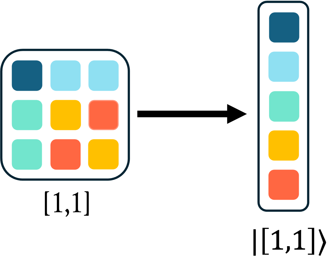
Take \(N=2\), one exponential per molecule, and \(L=2\). The six conventional labels are \((0,0)\), \((1,0)\), \((0,1)\), \((2,0)\), \((1,1)\), and \((0,2)\). Each carries a \(3\times3\) ADO: 54 complex entries. Relabeling the two molecules leaves four canonical labels, so a first reduction gives 36 entries. Their matrices contain, respectively, 5, 9, 9, and 5 distinct entries: the final calculation propagates only 28 complex variables. We will construct all four matrices explicitly in Section 16.
For fixed \(m\) and \(L\), the canonical-label count stops increasing once \(N\geq L\). The unique-variable count stops increasing once \(N\geq L+2\). The extra two molecules are needed to represent the distinction between a diagonal entry and a coherence between two different molecules in the zero-occupation category.
The word “exact” refers first to an algebraic statement: the compressed equations reproduce the same finite HEOM problem, with the same bath expansion, hierarchy closure, Hamiltonian, and initial condition. Convergence of that finite problem to the intended physical model is a separate question. In particular, a fixed number of propagated variables does not imply that the physical dynamics have become independent of \(N\).
Primary source: Mondal and Huo, arXiv:2608.20657v2, abstract and Sections I–V. This tutorial follows the supplied v2 article. Intermediate algebra, the small-system validation program, and the exercises are teaching additions, not additional numerical results from the paper.
2. Start with the states and the tensor-product spaces
Let \(\mathcal H_{\rm cav}\) be the cavity Fock space and \(\mathcal H_i=\operatorname{span}\{|g_i\rangle,|e_i\rangle\}\) the electronic space of molecule \(i\). Before restricting the excitation number, the system space is
The cavity operators are \(\hat a\) and \(\hat a^\dagger\). On molecule \(i\), define \(\hat\sigma_i^+=|e_i\rangle\langle g_i|\) and \(\hat\sigma_i^-=|g_i\rangle\langle e_i|\). Identity operators on spectator factors are understood only in this full-space expression:
We use \(\hbar=1\) throughout. Thus energies and angular frequencies have the same units, and time has the reciprocal unit. The rotating-wave approximation keeps exchange terms that conserve \(\hat N_{\rm ex}=\hat a^\dagger\hat a+\sum_i\hat\sigma_i^+\hat\sigma_i^-\). Counter-rotating terms, such as \(\hat a^\dagger\hat\sigma_i^+\), are not in this Hamiltonian.
The one-excitation states, including their spectator factors, are
The ordered basis used for every system matrix below is \(\mathcal B_N=(|c\rangle,|e_1\rangle,\ldots,|e_N\rangle)\) unless another basis is stated. In this basis,
There is no direct intermolecular hopping in this particular model. All molecular excitation energies are the same, and \(g\) is a real, identical molecule–cavity coupling. Those assumptions will later make molecular relabeling a symmetry.
For example, for two molecules, \([\hat Q_1]_{\mathcal B_2}=\operatorname{diag}(0,1,0)\) and \([\hat Q_2]_{\mathcal B_2}=\operatorname{diag}(0,0,1)\). These operators act on the system, not on the environmental oscillators. Let \(\mathcal H_B=\bigotimes_i\mathcal H_{B_i}\) denote the bath space. On \(\mathcal H_S^{(1)}\otimes\mathcal H_B\), the total Hamiltonian is explicitly
The distinction between the two factors is important: an ADO is a system-space operator that encodes environmental information. It is not a matrix containing both electronic and oscillator basis indices.
Model and conventions: paper Section II A–B, Eqs. (2)–(10).
3. Why a two-state bright–cavity model is not enough
The normalized bright exciton is \(|B\rangle=N^{-1/2}\sum_i|e_i\rangle\). Choose \(N-1\) orthonormal dark kets \(|D_\alpha\rangle\) satisfying \(\langle B|D_\alpha\rangle=0\). Acting with the Hamiltonian on the bright ket gives
The second identity follows because the molecular amplitudes of a dark ket sum to zero. In the ordered basis \(\mathcal B_{BD}=(|c\rangle,|B\rangle,|D_1\rangle,\ldots)\),
The two polariton energies are obtained by setting the determinant of the \(2\times2\) block minus \(E\hat I_2\) to zero:
Choose \(g\geq0\) by a phase convention. Define \(2\theta=\operatorname{atan2}(2g\sqrt N,\Delta)\), with \(0\leq\theta\leq\pi/2\). Unlike a bare tangent formula, this specifies the quadrant away from resonance. Then
On resonance, \(\theta=\pi/4\) and the splitting is \(\Omega_R=2g\sqrt N\). The system Hamiltonian therefore has a simple bright–cavity block. The environment does not share that block structure.
Two molecules: write the bath projectors in the collective basis
For \(N=2\), choose \(|B\rangle=(|e_1\rangle+|e_2\rangle)/\sqrt2\) and \(|D\rangle=(|e_1\rangle-|e_2\rangle)/\sqrt2\). The change-of-basis matrix has the new basis kets as its columns in \(\mathcal B_2\):
Consequently, \(\langle B|\hat H_{SB}|D\rangle=(\hat B_1-\hat B_2)/2\). Its thermal mean is zero, but its correlation is not zero. The difference between the two independent local bath forces couples bright and dark states.
A permutation-invariant density operator need not be supported only on permutation-invariant kets. For example, \(|D\rangle\) changes sign when two molecules are exchanged, but \(|D\rangle\langle D|\) does not. For general \(N\), the normalized dark mixture \(\hat P_D/(N-1)\) is invariant, where
This is why a symmetric density operator can acquire dark population without breaking the symmetry used for compression. Symmetry adaptation is not a projection onto the bright ket alone.
Bright and polariton definitions: paper Eqs. (4)–(6). The explicit two-molecule basis transformation is a worked example.
4. Derive the bath correlation function
Each molecular bath consists of harmonic oscillators. Write \(\hat H_B=\sum_{i\xi}\omega_\xi\hat b_{i\xi}^\dagger\hat b_{i\xi}\) and, with real coupling amplitudes for simplicity, \(\hat B_i=\sum_\xi f_\xi(\hat b_{i\xi}+\hat b_{i\xi}^\dagger)\). The index \(\xi\) labels actual oscillator modes; it is not the exponential index \(k\) introduced later.
The reference initial state is factorized:
For one oscillator, the thermal occupation is \(\bar n_\xi=(e^{\beta\omega_\xi}-1)^{-1}\). The only nonzero second moments needed here are \(\langle\hat b_\xi^\dagger\hat b_\xi\rangle=\bar n_\xi\) and \(\langle\hat b_\xi\hat b_\xi^\dagger\rangle=\bar n_\xi+1\). Under free bath evolution,
Substitute these into \(\langle\hat B_i(t)\hat B_j(0)\rangle_B\). Independence eliminates cross-molecule terms, while independence of the modes eliminates cross-mode terms. Thus
The identity \(2\bar n_\xi+1=\coth(\beta\omega_\xi/2)\) and the spectral-density convention \(J(\omega)=\pi\sum_\xi|f_\xi|^2\delta(\omega-\omega_\xi)\) give
The real part is the symmetrized fluctuation correlation. The imaginary part is half the bath commutator divided by \(i\) and carries the bath-response information. It should not be discarded merely because the bath has zero mean. Replacing a quantum correlation by a purely real classical noise correlation is a change of physical model, not a consequence of molecular symmetry.
“Identical independent baths” means the same function \(C(t)\) for every molecule, with \(\delta_{ij}\) between molecules. “One common bath” would instead have nonzero cross correlations between different molecules. These are different problems.
Bath definition and spectral convention: paper Eqs. (7)–(12).
5. Exponential channels, complex conjugation, and the Drude example
HEOM closes an infinite chain of first-order equations when the bath correlation is written as a sum of exponentials. For the retained correlation, choose
Both equations use the same ordered set of rates. If every \(\nu_k\) is real, then \(\check c_k=c_k^*\). For complex rates, this shortcut is generally wrong. Let \(\bar k\) be the conjugate partner satisfying \(\nu_{\bar k}=\nu_k^*\). Relabeling the terms in \(C_m^*(t)=\sum_k c_k^*e^{-\nu_k^*t}\) gives \(\check c_k=c_{\bar k}^*\).
A damped oscillatory contribution
Take \(C(t)=A e^{-(\gamma+i\Omega)t}+B e^{-(\gamma-i\Omega)t}\). In the rate order \((\gamma+i\Omega,\gamma-i\Omega)\), the forward coefficients are \((A,B)\), while the coefficients for \(C^*\) are \((B^*,A^*)\). This partner exchange must be retained in the downward HEOM terms. A conjugate pair is two exponential channels, not two distinguishable molecules.
The one-exponential Drude contribution
For \(J_{\rm DL}(\omega)=2\lambda\gamma\omega/(\omega^2+\gamma^2)\), \(\lambda\) is the reorganization energy and \(\gamma\) the bath decay rate. Evaluating the thermal correlation by its Drude pole and thermal poles gives, for positive time,
The first line is one exponential. The full finite-temperature Drude correlation generally also needs the second line, a different controlled decomposition, or a justified residual correction. When \(\beta\gamma\ll1\), expanding \(\cot x=1/x-x/3+\cdots\) gives \(c_0\simeq2\lambda/\beta-i\lambda\gamma\). This is a high-temperature approximation to the coefficient, not the definition of the entire exact quantum correlation.
A useful way to understand a fast-residual terminator is to define the omitted real correlation \(\delta C_R(t)\) and its one-sided integral \(\Delta_R=\int_0^\infty\delta C_R(t)\,dt\). If the system changes little over the residual correlation time, replace a convolution by
This produces the time-local addition
The definition by the one-sided integral avoids ambiguous factors of two associated with delta functions at an integration endpoint. If only the exact Drude pole is retained and every positive Matsubara term is assigned to this residual,
This expression assumes that exact pole coefficient, rather than its high-temperature replacement. The residual approximation and the terminal-tier closure are also different operations: one handles omitted bath-correlation components; the other handles omitted high-tier ADOs. The paper uses an Ishizaki–Tanimura residual correction in its one-exponential numerical examples. Symmetry reduction preserves a compatible correction but does not make the correction itself exact.
Finally, keep the energy convention consistent. A displaced oscillator can introduce a reorganization counterterm proportional to \(\sum_i\hat Q_i\). Here \(\epsilon_x\) means the energy actually used in \(\hat H_S\). Do not add or subtract \(\lambda\) a second time because another implementation uses a different definition of its input excitation energy.
Channel pairing: paper Eq. (12). Drude parameters and residual correction: paper Section VII. For broader HEOM background, see Tanimura, J. Chem. Phys. 153, 020901 (2020).
6. Derive the hierarchy from exponential memory
It is tempting to regard an ADO as a density matrix for a molecule with an extra bath excitation. That interpretation is not generally correct. A hierarchy occupation counts the order of a memory functional. It need not equal the occupation of any physical oscillator.
For linear coupling to a harmonic bath initially in a Gaussian thermal state, all connected bath correlations above second order vanish. After tracing the bath on the forward and backward evolution branches, its influence can therefore be written using \(C(t)\) alone. The following derivation makes the hierarchy-generating step explicit.
Forward and backward histories
Use system paths in the basis that diagonalizes all \(\hat Q_i\). Let \(q_i^+(s)\) and \(q_i^-(s)\) be their eigenvalues on the forward ket and backward bra paths at time \(s\). They are scalar history functions, not operators. The bath influence functional is
The system Hamiltonian can be nondiagonal in this basis; its transitions are included in the system path weight. Gaussianity closes the bath cumulant expansion. It does not replace the system operators by commuting numbers in the original Schrödinger equation.
For each molecule and exponential channel, define the scalar memory functional
Differentiate this integral. The upper-limit contribution evaluates the integrand at \(u=t\), and the derivative of its exponential contributes \(-\nu_k\mathcal I_{ik}\):
Meanwhile, differentiating the upper endpoint of the influence exponent gives
The signs can be checked directly: \(-i\mathcal I_{ik}\) equals minus the corresponding correlation convolution because \((-i)(-i)=-1\).
Define the auxiliaries and use the product rule
For a hierarchy label \(n=(n_{10},\ldots,n_{N,m-1})\) of nonnegative integers, define \(\hat\rho_n(t)\) by the same forward–backward path integral as the reduced density operator, but insert \(\prod_{ik}\mathcal I_{ik}^{n_{ik}}\) into its integrand. Schematically, with \(\mathcal W_S\) including both system propagators, boundary conditions, and the initial system density operator,
The zero powers give \(\hat\rho_0=\hat\rho_S\). There are three contributions to its general derivative. Differentiating the system weight gives \(-i[\hat H_S,\hat\rho_n]\). Differentiating \(\mathcal F\) inserts one additional \(\mathcal I_{ik}\), which raises \(n_{ik}\) by one. Differentiating one of the \(n_{ik}\) identical memory factors lowers its power by one and produces the integer factor \(n_{ik}\).
The damping pieces add to \(\Gamma_n=\sum_{ik}n_{ik}\nu_k\). At a final-time endpoint, multiplication by \(q_i^+\) becomes left multiplication by \(\hat Q_i\), and multiplication by \(q_i^-\) becomes right multiplication by \(\hat Q_i\). With \(e_{ik}\) denoting a unit shift of the hierarchy label, the result is
A downward term with \(n_{ik}=0\) is absent. At \(t=0\), every memory integral vanishes, so a factorized thermal preparation has \(\hat\rho_n(0)=0\) whenever \(|n|=\sum_{ik}n_{ik}>0\). A correlated initial equilibrium preparation need not have this property: its bath history is already encoded in nonzero auxiliaries.
These are local-in-time equations in an enlarged space. The physical density operator alone is still non-Markovian because its derivative depends on the first tier, whose derivative depends on further tiers. The auxiliary hierarchy stores the memory that a reduced equation would otherwise express through time integrals.
This influence-functional derivation supplies the intermediate steps leading to the conventional hierarchy used in paper Section II C. Its assumptions are a Gaussian harmonic bath, linear coupling, the stated bath preparation, and the specified exponential correlation representation.
7. Scale the auxiliaries and write an explicit Liouville matrix
The factorials generated by repeated differentiation can make unscaled ADO magnitudes vary strongly with tier. Introduce the positive scalar
For the simple scaling below, retained channels have nonzero \(|c_k|\). A representation with a vanishing forward coefficient but a nonvanishing partner needs a nonsingular scaling choice instead of division by zero.
Substitute \(\hat\rho_n=s_n\tilde{\hat\rho}_n\) into the unscaled equation and divide by \(s_n\). The upward ratio and downward ratio are
The factorial ratio supplies \(n_{ik}+1\) upward and \(1/n_{ik}\) downward. Therefore
This is a change of coordinates, not a new dynamical approximation. A hard total-tier cutoff retains \(|n|\leq L\) and sets the upward connection out of tier \(L\) to zero. Other closures must be specified separately.
A one-molecule, two-state example
Let \(\mathcal B_1=(|c\rangle,|e_1\rangle)\) and vectorize by stacking columns. The ordered Liouville basis is \((|c\rangle\langle c|,|e_1\rangle\langle c|,|c\rangle\langle e_1|,|e_1\rangle\langle e_1|)\). Thus
Here a double ket denotes a coordinate vector for an operator, not a physical pure state. The identity \(\operatorname{vec}(\hat A\hat X\hat B)=(\hat B^{\mathsf T}\otimes\hat A)\operatorname{vec}(\hat X)\) gives the Hamiltonian superoperator
The transpose is not a Hermitian adjoint: it comes from column vectorization of right multiplication. In the same ordered Liouville basis,
For one real-rate exponential and \(L=2\), stack the three four-component ADO vectors in the order \(n=0,1,2\). The entire 12-dimensional generator is the block matrix
Every symbol in this block matrix is now an explicit \(4\times4\) matrix. The top-tier upward block is absent because of the hard cutoff. Multiple molecules add hierarchy directions; molecular symmetry will identify repeated directions without changing this underlying structure.
Scaling and finite hierarchy: paper Eqs. (14)–(18). The explicit Liouville matrices are derived here in column-stacking order.
8. Count the conventional hierarchy before compressing it
There are \(K=Nm\) hierarchy directions. At an exact tier \(\ell\), a label is a nonnegative integer solution of \(n_1+\cdots+n_K=\ell\). A stars-and-bars argument places \(K-1\) dividers among \(\ell\) occupations, giving \(\binom{K+\ell-1}{\ell}\) labels.
To count all tiers at once, introduce the unused-depth variable \(n_{K+1}=L-\sum_{j=1}^{K}n_j\). It is nonnegative and makes the total exactly \(L\). The same counting argument now gives
For complex double precision, one stored state vector uses \(16D_{\rm full}\) bytes. This excludes derivative arrays, integration stages, indexing tables, and the program itself. It is a useful lower bound, not a peak-memory estimate.
For fixed \(L\) and \(m\), the leading large-\(N\) behavior is \(N_{\rm ADO}^{\rm full}\sim(Nm)^L/L!\). Multiplying by the dense system matrix makes the raw variable count scale as \(N^{L+2}\). This is why even a system Hamiltonian with only \(O(N)\) nonzero entries does not, by itself, solve the conventional HEOM memory problem.
Conventional counts: paper Eqs. (17)–(18).
9. Prove the relabeling relation—and check the initial state
A molecular relabeling \(\pi\) is represented on the system by the unitary permutation operator \(\hat U_\pi|c\rangle=|c\rangle\) and \(\hat U_\pi|e_i\rangle=|e_{\pi(i)}\rangle\). Identical molecular parameters imply
A molecule carries its entire bath-channel history with it. For a multi-exponential label, define \((\pi n)_{ik}=n_{\pi^{-1}(i),k}\). The rate index \(k\) is unchanged. This preserves the total tier, damping, and neighbor structure:
For the Hamiltonian part, insert \(\hat U_\pi^\dagger\hat U_\pi=\hat I\) between the factors and use the invariance of \(\hat H_S\). For the upward part, transform \(\hat Q_i\) and rename the summed molecular index. The downward part transforms in the same way because \(c_k\), \(\check c_k\), and \(\nu_k\) do not depend on \(i\). Therefore, if \(\{\tilde{\hat\rho}_n(t)\}\) is a solution, then
is also a solution, but generally with relabeled initial data. This is covariance. It does not yet let us identify two ADOs within the same calculation.
For that identification, require \(\tilde{\hat\rho}_{\pi n}(0)=\hat U_\pi\tilde{\hat\rho}_n(0)\hat U_\pi^\dagger\). The original and relabeled hierarchies then satisfy the same finite linear initial-value problem. Uniqueness of its solution gives
For a factorized preparation, all nonzero-tier initial ADOs vanish, so the remaining condition is \(\hat U_\pi\hat\rho_S(0)\hat U_\pi^\dagger=\hat\rho_S(0)\). Cavity, bright, and polariton populations satisfy it. A localized population \(|e_1\rangle\langle e_1|\) does not satisfy it for an exchange involving molecule 1.
Two molecules and a first-tier ADO
In \(\mathcal B_2\), the exchange operator and the first-tier relation are
If the stored matrix has entries \(\begin{pmatrix}z&a&b\\d&p&s\\f&t&r\end{pmatrix}\), its relabeled partner is \(\begin{pmatrix}z&b&a\\f&r&t\\d&s&p\end{pmatrix}\). They are related matrices, not necessarily identical arrays. This distinction is the reason alignment is essential after canonicalization.
Covariance proof and preparation condition: paper Eqs. (19)–(27) and the discussion immediately following them.
10. First reduction: store one canonical occupation pattern
Start with one exponential per molecule, so a label is \(n=(n_1,\ldots,n_N)\). Sort the positive occupations in descending order and suppress the zeros. The result is a canonical pattern \(\Lambda=[\Lambda_1,\ldots,\Lambda_r]\), where \(\Lambda_1\geq\cdots\geq\Lambda_r>0\) and \(r\leq N\).
For storage, the representative molecule-resolved label is \(n^\Lambda=(\Lambda_1,\ldots,\Lambda_r,0,\ldots,0)\). Define \(\hat R_\Lambda=\tilde{\hat\rho}_{n^\Lambda}\). The empty pattern \(\varnothing\) is the physical density operator. No statistical averaging has been performed in this definition: \(\hat R_\Lambda\) is one representative, not a sum over all relabelings.
Let \(M_q^\Lambda\) be the number of molecules carrying occupation \(q\). Then
The number of conventional labels represented by \(\Lambda\) is
The numerator counts all assignments to molecular labels. Dividing by \(M_q!\) removes assignments that only exchange equal occupations. The zero category must be included.
\(N=4\) and \(\Lambda=[2,1]\)
The representative is \((2,1,0,0)\), with \(M_2=1\), \(M_1=1\), and \(M_0=2\). There are \(4!/(1!1!2!)=12\) distinct conventional labels. They include \((2,1,0,0)\), \((0,2,1,0)\), and \((1,0,0,2)\). Their matrices are reconstructed by molecular relabeling of one \(\hat R_{[2,1]}\).
Do not multiply \(\hat R_{[2,1]}\) itself by 12. This multiplicity counts conventional labels, not the normalization of the retained ADO. Factors entering the equations arise from actual sums of equal contributions, which will be derived separately.
At tier \(\ell\), the patterns are integer partitions of \(\ell\) with at most \(N\) parts. Writing this count as \(p_N(\ell)\),
Through \(L=3\), the unrestricted list is \(\varnothing\); \([1]\); \([2],[1,1]\); and \([3],[2,1],[1,1,1]\). There are seven patterns. A system with \(N=2\) excludes \([1,1,1]\), leaving six. Once \(N\geq L\), no partition through tier \(L\) is excluded, so the count becomes \(\sum_{\ell=0}^{L}p(\ell)\), independent of \(N\).
Canonical representatives and orbit sizes: paper Eqs. (28)–(41). Saturation of their count: Eqs. (51)–(52).
11. Canonicalization must preserve the matrix labels
A hierarchy term does two things at once: it changes a bath occupation and acts with the projector of the molecule whose occupation changed. Sorting the target occupations without keeping track of that molecule generally produces the wrong matrix entry.
Starting from \(n^\Lambda\), form the raw target \(m_i^\pm=n^\Lambda\pm e_i\). The word “raw” means the molecular identities have not been reordered. Sorting gives \(\Lambda_i^\pm=\operatorname{canon}(m_i^\pm)\). Let \(\pi_i^\pm\) carry the stored canonical ordering of that target back into the raw molecular ordering. The required target operator is
Lowering the first molecule in \([2,2]\)
With \(N=4\), start from \((2,2,0,0)\). Lower molecule 1 to get \((1,2,0,0)\). The stored target is \([2,1]\), represented as \((2,1,0,0)\). To recover the raw target, exchange molecular labels 1 and 2.
Consequently, the raw target entry with row \(|e_1\rangle\) and column \(|c\rangle\) is the occupation-1 cavity coherence of \(\hat R_{[2,1]}\), not its occupation-2 coherence. Similarly, the raw \((e_1,e_2)\) entry has occupation categories \((1,2)\), not \((2,1)\). A code that sorts only the hierarchy label would get both entries wrong.
For a single real-rate exponential, define \(\chi_L(\Lambda)=1\) when \(|\Lambda|<L\) and zero at the terminal tier. The canonical equation is
This already evolves only canonical ADOs. However, implementing it with full matrices would still store \((N+1)^2\) entries per pattern. The next reduction replaces the aligned matrix operation by direct access to one of a few distinct entries.
Raw targets, alignment, and the canonical equation: paper Eqs. (42)–(50).
12. Second reduction: identify the entries that are genuinely different
Suppose molecules \(i\) and \(j\) carry the same occupation in \(n^\Lambda\). Exchanging them leaves the hierarchy label unchanged. The covariance relation then implies \(\hat R_\Lambda=\hat U_{ij}\hat R_\Lambda\hat U_{ij}^\dagger\). A simultaneous exchange of those rows and columns cannot change the representative.
Let \(\mathcal G_\Lambda=\{q:M_q^\Lambda>0\}\) be the occupation categories actually present, with \(G_\Lambda=|\mathcal G_\Lambda|\). Do not include the zero category when no zero-occupation molecules remain. Every required matrix entry falls into one of the following types:
\(T_q\) exists only if \(M_q\geq2\). It is not the same variable as \(P_q\): relabeling cannot turn a diagonal entry into an off-diagonal one. \(S_{qr}\) is ordered, so \(S_{qr}\) and \(S_{rq}\) are both retained. Similarly, \(X_q\) and \(Y_q\) are separate complex coordinates.
For the physical Hermitian density operator, opposite coherences are complex conjugates. Individual auxiliaries need not have that simple relation for a general complex-rate representation. Even in a real-rate convention where Hermitian initial auxiliaries remain Hermitian, retaining both directions is a safe linear coordinate choice and permits non-Hermitian initial operators used in response calculations. The counts below do not exploit an additional Hermiticity reduction.
The complete \(N=4\), \([2,1]\) representative
In the ordered basis \((|c\rangle,|e_1\rangle,|e_2\rangle,|e_3\rangle,|e_4\rangle)\), with occupation assignment \((2,1,0,0)\),
There are 25 matrix entries but only 17 distinct complex variables. Molecules 3 and 4 share their cavity coherences and populations, but their mutual coherence remains a separate \(T_0\). At \(N=10\), this same pattern has 121 matrix entries and still only 17 distinct variables. The multiplicity of its zero category changes from 2 to 8.
For each pattern, define \(h_\Lambda=\#\{q:M_q^\Lambda\geq2\}\). Counting one \(Z\), three variables per category, ordered cross-category coherences, and the allowed \(T\) variables gives
The full propagated dimension is \(D_u=\sum_{|\Lambda|\leq L}u(\Lambda)\). This is a count of complex coordinates in a chosen linear representation, not a count of independent real parameters of a normalized density operator.
Variable definitions and example: paper Eqs. (53)–(69).
13. Why the second threshold is \(L+2\), not \(L\)
At fixed depth \(L\), every pattern has at most \(L\) nonzero occupations. Beyond \(N\geq L\), all patterns are already present. However, increasing \(N\) can still create a zero category where none existed, or give a formerly singleton zero category a second molecule. The latter creates the new variable \(T_0\).
Once \(M_0^\Lambda=N-r\geq2\) for every retained pattern, neither change can occur. Because \(r\leq L\), the sufficient uniform threshold is \(N\geq L+2\). Above it,
There can be earlier saturation for a particular pattern or a specially restricted calculation; \(L+2\) is the general bound for this full family of one-excitation density operators. The underlying reason is structural: a matrix entry can involve zero, one, or two distinct molecular identities.
At \(L=25\), direct enumeration of the patterns gives 9,296 canonical ADOs for \(N\geq25\). The exact unique-variable counts near the second threshold are:
| Molecules \(N\) | Canonical ADOs | Unique complex variables | One vector, decimal MB |
|---|---|---|---|
| 25 | 9,296 | 306,743 | 4.907888 |
| 26 | 9,296 | 306,750 | 4.908000 |
| 27 | 9,296 | 306,751 | 4.908016 |
| \(10^{12}\) | 9,296 | 306,751 | 4.908016 |
The storage is \(16D_u\) bytes. These values exclude runtime connection arrays, integrator workspaces, and all other process memory. The statement is that the state-vector size has saturated—not that the entire executable occupies 4.91 MB.
Explore the exact counts
One exponential per local bath; fully permutation-symmetric operator; hard total-tier cutoff. The conventional counts below use integer arithmetic, not floating-point extrapolation.
Supported here: \(1\leq N\leq10^{12}\) and \(0\leq L\leq25\). Enter N using digits only
(for example, 1000000000000),
without commas or scientific notation.
This is a combinatorial calculator, not a runtime benchmark.
The default calculation has 9,296 canonical ADOs and 306,751 unique variables, requiring 4.908016 MB for one complex-double vector. Enable JavaScript to change the parameters.
Saturation proof: paper Eqs. (70)–(72). The exact \(L=25\) counts are also reported in Section VII E and are independently checked by the companion program.
14. Derive the Hamiltonian action without reconstructing matrices
Compression is useful only if the derivative can be evaluated in the compressed coordinates. Let \(q\) be the category of molecule \(i\). The molecular part of row \(i\) contains its own diagonal entry, \(M_q-1\) equivalent off-diagonal entries in the same category, and \(M_r\) entries in every other category. Therefore define the scalar row and column sums
When \(M_q=1\), omit the \(T_q\) term rather than accessing an undefined variable. For \([2,1]\) at \(N=4\), \(\mathfrak r_0=P_0+T_0+S_{02}+S_{01}\). At \(N=10\), it becomes \(P_0+7T_0+S_{02}+S_{01}\).
Derive a cavity–molecule equation entry by entry
For \(X_q=\langle e_i|\hat R_\Lambda|c\rangle\), the two products in the commutator are
Subtract them, multiply by \(-i\), and add the hierarchy damping \(-\Gamma_\Lambda X_q\). This gives \(\dot X_q|_{H+\Gamma}=-i(\epsilon_x-\omega_{\rm cav})X_q-ig(Z-\mathfrak r_q)-\Gamma_\Lambda X_q\). Repeating the same multiplication for all variable types yields the complete set:
For a molecular off-diagonal entry \((i,j)\), the two equal electronic energies cancel, leaving only \(gY_r-gX_q\). This explains the last two equations. Their equality of form does not make \(P_q\) and \(T_q\) redundant: their hierarchy couplings differ.
For one exponential, \(\Gamma_\Lambda=\nu|\Lambda|\). With multiple channels, \(\Gamma_\Lambda\) is the sum of the occupied local rates. The Hamiltonian equations themselves keep the same category structure.
Only the grouped sums require more than one or two terms. They run over the categories present in the pattern, not over the \(N\) molecules. A million equal contributions are represented by one variable multiplied by its multiplicity.
Grouped sums and representative component equations: paper Eqs. (75)–(81). The remaining component equations are derived explicitly here.
15. Derive the hierarchy action one matrix entry at a time
The local projector \(\hat Q_i=|e_i\rangle\langle e_i|\) makes the hierarchy action especially simple. For a matrix entry \(A_{ab}=\langle a|\hat A|b\rangle\),
Only a bath attached to the row or the column molecule can contribute. For a cavity–cavity entry neither contributes. A molecular diagonal entry has the same row and column molecule, so its upward commutator cancels exactly.
Define \(\mathcal A_i^\pm(a,b)\) as the aligned target entry with raw label \(m_i^\pm\) and canonical pattern \(\Lambda_i^\pm\). It is a scalar accessor, not an additional propagated object. For a one-exponential real-rate bath, set
For any source variable \(V_{ab}^\Lambda=\langle a|\hat R_\Lambda|b\rangle\), the hierarchy contribution is
Although this formula displays a sum over molecules, at most two distinct molecular labels survive. When several exponential channels are retained, repeat the same row and column logic for each channel.
Cavity and cavity–molecule entries
For \(Z\), all deltas vanish: \(\dot Z|_{\rm hier}=0\). For \(X_q\) and \(Y_q\), choose a molecule \(i\) of occupation \(q\) and obtain
A downward term at \(q=0\) is absent; the notation \(b_0=0\) must not cause a program to request a nonexistent negative-occupation target.
Diagonal and off-diagonal molecular entries
For a population-type coordinate, row and column are the same molecule. The upward pieces cancel, but the two coefficients in the downward term need not cancel:
At the physical tier \(q=0\), this is zero. Local diagonal coupling therefore has no direct term in the site population derivative. Population relaxation still occurs through the Hamiltonian and the bath-modified coherences.
For \(S_{qr}\), choose distinct molecules \(i\) and \(j\) with occupations \(q\) and \(r\). Then
The equation for \(T_q\) is the same expression with \(r=q\) but still \(i\ne j\). It does not reduce to the population equation: raising the row molecule and raising the column molecule access different entries of the target representative.
Follow the variables when a category changes
At \(N=4\), \(\Lambda=[2,1]\), consider \(S_{20}=\langle e_1|\hat R_{[2,1]}|e_3\rangle\). Raising the row molecule gives raw label \((3,1,0,0)\), pattern \([3,1]\), and target entry \(S_{30}^{[3,1]}\). Raising the column molecule gives \((2,1,1,0)\), pattern \([2,1,1]\), and target entry \(S_{21}^{[2,1,1]}\). Lowering the row molecule gives \((1,1,0,0)\) and \(S_{10}^{[1,1]}\); the zero-occupation column cannot be lowered. Hence, for \(L\geq4\),
At \(L=3\), both upward terms are removed. No factor \(M_0=2\) multiplies the column term: this particular matrix element selects one column molecule, not the sum of both zero-category molecules.
An accessor that avoids permutation matrices
Keep the raw target occupations attached to their molecular labels long enough to inspect the requested row and column. Then identify the target variable from their new categories: cavity/cavity means \(Z\); molecule/cavity means \(X\); cavity/molecule means \(Y\); identical molecular labels mean \(P\); different labels in the same category mean \(T\); different categories mean ordered \(S\). Only the target pattern is sorted to find its stored location.
This procedure is equivalent to applying \(\hat U_\pi\hat R\hat U_\pi^\dagger\), but it does not construct \(\hat U_\pi\) or \(\hat R\). It also handles a lowering move that merges two categories and a raising move that splits a category.
Aligned access and sparse row/column selection: paper Eqs. (82)–(89). The explicit component specialization and target-tracing example are derived here.
16. A complete two-molecule hierarchy through \(L=2\)
Let \(N=2\), \(m=1\), and \(L=2\). Store the patterns in the order \(\varnothing,[1],[2],[1,1]\). In the same system basis \(\mathcal B_2=(|c\rangle,|e_1\rangle,|e_2\rangle)\), their matrices are
The local dimensions are \(5+9+9+5=28\). The subscripts are occupation categories, not molecule numbers: \(P_1^{[1,1]}\) describes either molecular population entry, whereas \(P_1^{[1]}\) describes only the molecule carrying one hierarchy occupation.
For the physical block, define the bookkeeping ket \(|r_0\rangle=(Z,X_0,Y_0,P_0,T_0)^{\mathsf T}\). Its Hamiltonian action is the following \(5\times5\) matrix in that explicitly stated coordinate order:
The physical block has zero hierarchy damping. Its hierarchy contribution is
This is an explicit demonstration of bath-mediated dark-state dynamics. Without the hierarchy, \(P_0\) and \(T_0\) have identical derivatives. With the hierarchy, \(T_0\) has an extra term while \(P_0\) does not. Their difference, which determines dark population, can therefore grow.
As a first-tier example, \(X_1^{[1]}\) has a downward contribution \(-icX_0^{\varnothing}/\sqrt{|c|}\) and an upward contribution \(-i\sqrt{2|c|}X_2^{[2]}\). The coherence \(X_0^{[1]}\) has no downward contribution from its zero-occupation row, but its upward target is \(X_1^{[1,1]}\). These two distinct first-tier coherences would be incorrectly merged by a bright-only approximation.
All derivatives of the remaining 23 coordinates follow directly from Sections 14–15. The companion program constructs those coefficients and verifies the resulting 28-dimensional representation against the full 54-entry hierarchy.
17. Recover physical observables from five numbers
For a fully symmetric physical density operator with \(N\geq2\), the empty pattern has only the zero category. Suppress its superscript and write the five variables as \(Z,X,Y,P,T\). The trace and total site population are immediately
The bright population is a sum over all ordered molecular matrix entries. There are \(N\) diagonal terms and \(N(N-1)\) off-diagonal terms. Dividing by the bright-state normalization gives
Subtract bright population from total exciton population to obtain
This is the population summed over all \(N-1\) dark states. It is not the population of one chosen dark ket. The scalar \(T\) can be positive, negative, or complex in a general operator calculation; for the physical Hermitian symmetric density operator it is real.
The full collective-basis density matrix
Within the molecular sector, the matrix is \((P-T)\hat I_N+T\hat J_N\), where \(\hat J_N\) has every entry equal to one in the site basis. The bright ket is an eigenvector of \(\hat J_N\) with eigenvalue \(N\), while every dark ket has eigenvalue zero. In the collective basis introduced in Section 3,
This block form makes the distinction between Hilbert-space and operator symmetry especially clear. The dark block is present even though every molecule is equivalent. For a physical density operator, positivity can be checked without diagonalizing an \((N+1)\times(N+1)\) matrix: require \(P-T\geq0\) and the \(2\times2\) bright–cavity block to be positive semidefinite. In particular, \(Z\geq0\), \(P_B\geq0\), and \(ZP_B-N|X|^2\geq0\), with \(Y=X^*\).
Using the polariton kets, expand each quadratic form:
Adding them cancels the coherence terms. Hence \(P_++P_-+P_D=Z+NP\), which must remain one in the no-loss calculation. The trace derivative cancels directly: \(\dot Z|_H=-igN(X-Y)\) and \(N\dot P|_H=+igN(X-Y)\), while the physical diagonal hierarchy terms vanish.
Initialize the state in the same coordinate convention
Factorized preparation sets every nonempty pattern to zero. The physical variables for several useful initial states are
| Initial operator | \(Z\) | \(X=Y\) | \(P=T\) |
|---|---|---|---|
| \(|c\rangle\langle c|\) | 1 | 0 | 0 |
| \(|B\rangle\langle B|\) | 0 | 0 | \(1/N\) |
| \(|+\rangle\langle+|\) | \(\cos^2\theta\) | \(\sin\theta\cos\theta/\sqrt N\) | \(\sin^2\theta/N\) |
| \(|-\rangle\langle-|\) | \(\sin^2\theta\) | \(-\sin\theta\cos\theta/\sqrt N\) | \(\cos^2\theta/N\) |
An incoherent equal mixture of sites instead has \(Z=X=Y=T=0\) and \(P=1/N\). Its bright population is \(1/N\) and its dark population is \((N-1)/N\), unlike a pure bright state whose dark population is zero. Equal site populations alone do not determine whether the excitation is bright.
For \(N=1\), there is no dark sector and no \(T\) coordinate. Use \(P_B=P\) and \(P_D=0\) rather than requesting a nonexistent \(T_0\).
Observables and symmetric preparations: paper Eqs. (90)–(101). The collective-basis block form and positivity check are derived from those variables here.
18. Localized states do not destroy all of the symmetry
The initial operator \(|e_1\rangle\langle e_1|\) singles out molecule 1. A permutation exchanging it with molecule 2 changes the initial condition, so the fully symmetric five-variable physical block is not sufficient. But exchanges among molecules \(2,\ldots,N\) still leave the initial operator unchanged.
Keep the distinguished molecular label, its system row and column, and its local hierarchy occupation explicit. Canonicalize only the remaining \(N-1\) molecules. For one exponential, a partially symmetric hierarchy label has the form \((n_d;\Lambda)\) with \(n_d+|\Lambda|\leq L\).
One distinguished molecule and two equivalent spectators
For \(N=3\), in the ordered basis \((|c\rangle,|e_1\rangle,|e_2\rangle,|e_3\rangle)\), a physical operator invariant under exchange of molecules 2 and 3 has the structure
There are ten complex coordinates. For \(|e_1\rangle\langle e_1|\), set \(P_d=1\) and all other coordinates to zero. The same ten-coordinate physical structure handles a coherent cavity–site superposition; its initial values change, but its symmetry does not.
More generally, keep \(d\) distinguished molecules fixed and compress \(N-d\) others. The sufficient saturation thresholds become
For a particular partially symmetric pattern with \(G\) categories among the equivalent molecules, the coordinate count is \((d+G+1)^2+h\), where \(h\) counts equivalent categories with at least two members. Each distinguished molecule is a separate singleton category even when its hierarchy occupation equals that of another molecule.
Understand the localized state's initial collective populations
Because \(\langle B|e_1\rangle=1/\sqrt N\), a localized state has bright weight \(1/N\) and dark weight \(1-1/N\). On resonance,
For a more general normalized ket \(|\psi\rangle=a|c\rangle+b|e_1\rangle\), with \(|a|^2+|b|^2=1\), the resonant populations are
The initial UP–LP imbalance is an interference term. It depends on the relative phase of \(a\) and \(b\), not just on their populations. The paper's real-amplitude example \(a=\sqrt{0.7}\), \(b=\sqrt{0.3}\) gives \(P_\pm(0)=0.35+0.15/N\pm\sqrt{0.21/N}\) and \(P_D(0)=0.3(1-1/N)\).
Arbitrary initial operators from a small set of representative propagations
For a fixed factorized bath preparation, let \(\hat{\mathcal G}_t\) be the reduced dynamical map. Expand an arbitrary initial operator in the site/cavity matrix-unit basis:
Linearity propagates each term independently. Covariance gives \(\hat{\mathcal G}_t[\hat U_\pi\hat A\hat U_\pi^\dagger]=\hat U_\pi\hat{\mathcal G}_t[\hat A]\hat U_\pi^\dagger\). Therefore the five representative operator types are \(|c\rangle\langle c|\), \(|e_1\rangle\langle c|\), \(|c\rangle\langle e_1|\), \(|e_1\rangle\langle e_1|\), and \(|e_1\rangle\langle e_2|\). They distinguish zero, one, one, one, and two molecular labels.
When the bath-channel pairing and closure preserve adjoints, the responses to the two cavity–molecule orientations are adjoints and only four independent representative propagations are necessary. The non-Hermitian representatives are basis operators, not individually physical density matrices.
This statement concerns the number of representative dynamics. Reading an arbitrary dense input or writing all \((N+1)^2\) output entries still costs at least quadratic storage and work. Correlated initial system–bath states also require specifying their initial hierarchy, not merely the initial reduced density matrix.
Distinguished molecules and linear reconstruction: paper Section VI, Eqs. (94)–(115) and Table I. Coherent-state initial populations: Section VII C.
19. Multiple exponentials: move the entire local history together
With \(m\) exponential components, a molecule carries the ordered local occupation tuple \(\alpha_i=(n_{i0},\ldots,n_{i,m-1})\). These are bookkeeping labels, not oscillator wavefunctions. A molecular exchange moves the complete tuple. It must not independently sort or exchange its components.
A canonical pattern is now a multiset of nonzero local tuples, sorted by any fixed deterministic ordering. One convenient rule is decreasing total occupation, with lexicographic ordering to resolve ties. Include the zero tuple as a category whenever unoccupied molecules remain. If \(M_\alpha\) is the number of molecules in category \(\alpha\),
The unique-variable types remain \(Z\), \(X_\alpha\), \(Y_\alpha\), \(P_\alpha\), ordered \(S_{\alpha\beta}\), and \(T_\alpha\). Their count is still \((G+1)^2+h\). Changing channel \(k\) on one molecule changes its local category from \(\alpha\) to \(\alpha\pm e_k\), then the target multiset is canonicalized and the selected matrix entry is accessed in the raw labeling.
The general hierarchy contribution for a source entry \((a,b)\) is
There are at most two selected molecules for each \(k\). The Hamiltonian sums are unchanged except that their category indices are now tuples.
Enumerate every pattern for \(m=2\), \(L=2\)
Let \(A=(1,0)\) and \(B=(0,1)\). Tier zero contains only \(\varnothing\). Tier one contains \([A]\) and \([B]\). Tier two contains the three single-molecule patterns \([(2,0)]\), \([(1,1)]\), \([(0,2)]\), and the three two-molecule patterns \([A,A]\), \([A,B]\), \([B,B]\). This makes nine canonical patterns when \(N\geq2\).
For \(N\geq4\), the zero category always has at least two members. The unique-variable total is \(5+2(10)+3(10)+2(11)+17=94\). By comparison, one exponential at \(L=2\) has four canonical patterns and 36 saturated variables. Adding one exponential can therefore increase the compressed problem substantially even at shallow depth.
For \(\Lambda=[A,B]\) and two zero-category molecules, the block structure is the same 17-variable pattern as the \([2,1]\) example, with category labels \(A,B,0\). Raising channel 0 on the molecule in category \(B\) changes \(B=(0,1)\) to \((1,1)\); raising channel 1 instead changes it to \((0,2)\). They have the same total tier but different damping and target coefficients.
For completeness, the generating function for canonical tuple multisets is
The coefficient of \(z^r x^\ell\) counts patterns with \(r\) occupied molecules and total tier \(\ell\). At finite \(L\), only tuples of total occupation at most \(L\) can appear, so only finitely many factors matter. Restrict \(r\leq N\) and sum through \(\ell=L\).
Every nonzero local tuple still costs at least one tier. Therefore the canonical count saturates at \(N\geq L\), and the unique-variable count at \(N\geq L+2\), for fixed \(m\). The saturated size can grow rapidly with both \(m\) and \(L\). “Independent of ensemble size” does not mean independent of bath complexity.
The main article specifies the whole-tuple relabeling in Eqs. (21)–(23) and states the multi-exponential extension on page 12. The explicit enumeration and generating-function explanation are supplied here; the separate Supporting Information is not bundled in the supplied website archive.
20. Why Gaussian static disorder is a zero-rate channel
A fixed disordered realization has \(\hat H_S(\delta)=\hat H_S+\sum_i\delta\epsilon_i\hat Q_i\). Unless its site shifts happen to coincide, relabeling molecules changes that Hamiltonian. The fully symmetric generator cannot simply be applied to each individual realization.
The disorder average is a different object. Suppose \(\delta\epsilon_i=\sigma x_i\), where the \(x_i\) are independent standard Gaussian random variables, and the initial system operator is independent of the particular disorder realization. Their joint probability distribution is invariant under molecular relabeling. The averaged evolution can retain that covariance even though every sample breaks it.
The static random force has correlation \(\mathbb E[\delta\epsilon_i(t)\delta\epsilon_j(0)]=\delta_{ij}\sigma^2\). It is represented by the channel \(c_{\rm st}=\check c_{\rm st}=\sigma^2\), \(\nu_{\rm st}=0\). There is no damping along that hierarchy direction.
Derive this channel directly, without treating disorder as an oscillator
Let \(\phi_n(x)=\mathrm{He}_n(x)/\sqrt{n!}\) be the orthonormal probabilists' Hermite polynomials with respect to the standard Gaussian measure. Their recurrence is
For the conditional system operator \(\hat\rho_x(t)\), define polynomial-weighted disorder moments
Multiply \(\dot{\hat\rho}_x=-i[\hat H_S,\hat\rho_x]-i\sigma\sum_i x_i[\hat Q_i,\hat\rho_x]\) by the polynomial product and average. Apply the recurrence to the one factor containing \(x_i\). This yields
This is exactly the scaled hierarchy with \(c=\sigma^2\) and \(\nu=0\). Orthogonality gives \(\hat R_n(0)=0\) for nonzero \(n\) when the initial state is independent of the disorder. Additional dynamical-bath ADO labels can be carried alongside these polynomial labels.
Check the average against an elementary Gaussian integral
With no cavity coupling, a cavity–site coherence acquires the random phase \(e^{-i\delta\epsilon_i t}\). Gaussian averaging gives \(\mathbb E[e^{-i\delta\epsilon_i t}]=e^{-\sigma^2t^2/2}\). A coherence between two independently disordered sites has phase \(e^{-i(\delta\epsilon_i-\delta\epsilon_j)t}\) and decays as \(e^{-\sigma^2t^2}\). A converged zero-rate hierarchy should reproduce both laws.
A zero-rate channel can require a deep hierarchy over a long observation time because there is no tier damping to suppress its memory. Convergence must be checked over the full requested time interval. This is not the same numerical situation as a rapidly decaying Drude or Matsubara channel.
For non-Gaussian static disorder, a constant two-point correlation alone does not specify the distribution or its higher cumulants. The Gaussian HEOM channel cannot reproduce an arbitrary distribution merely by matching its variance. A suitable polynomial hierarchy may still be constructed from that distribution, but its recurrence coefficients and closure must be derived separately.
In the paper's disorder plots, upper, lower, and dark projectors refer to the mean disorder-free TC Hamiltonian. They are not redefined for each realization. This matters when interpreting the populations after disorder mixing.
Gaussian disorder and the static channel: paper Eqs. (124)–(126) and Fig. 7. The Hermite-moment derivation is a teaching addition.
21. Cavity loss: include the state that receives the photon
The one-excitation Hamiltonian conserves excitation number. Photon loss does not. To write a trace-preserving model, append the zero-excitation ket \(|G\rangle=|0\rangle_{\rm cav}\otimes|g_1\rangle\otimes\cdots\otimes|g_N\rangle\) and use the jump operator
The rate convention is now explicit: a bare cavity population decays at rate \(\kappa\), while a cavity amplitude decays at \(\kappa/2\). In the ordered basis \((|G\rangle,|c\rangle,|e_1\rangle,\ldots)\), the only nonzero matrix entry of \(\hat L_c\) is its ground-row/cavity-column entry \(\sqrt\kappa\).
For an arbitrary ADO, the jump term transfers its cavity entry to its ground entry. The anticommutator damps its cavity row and column. Thus
For molecular–molecular entries, this dissipator vanishes. Add the same system dissipator to every ADO when appending this independent Markovian loss channel. Since \(|G\rangle\) and \(|c\rangle\) are unchanged by molecular relabeling, the dissipator preserves the required covariance.
Without pumping or ground–excited driving, the excitation block evolves autonomously with the loss contributions \(\dot Z|_{\rm loss}=-\kappa Z\), \(\dot X_q|_{\rm loss}=-\kappa X_q/2\), and \(\dot Y_q|_{\rm loss}=-\kappa Y_q/2\). Its trace is a survival probability, not a normalized density-matrix trace:
One can recover the physical ground population from the lost trace in this no-return setting. In a full augmented hierarchy, the ground diagonal of each ADO has its own damping and the source \(\kappa Z^\Lambda\); it does not feed back into the excitation block without an additional excitation process.
Simply renormalizing the surviving excitation block after every step changes the question to conditional, postselected dynamics. That is not the unconditional loss dynamics above. Likewise, replacing \(\omega_{\rm cav}\) by a complex number without stating the associated bra evolution and jump treatment can hide a factor-of-two or normalization error.
The main article identifies cavity loss as a compatible extension in Section I. The explicit Lindblad block construction here is derived separately to specify the rate and normalization conventions.
22. Turn the derivation into a matrix-free program
Collect the unique coordinates of each pattern into a bookkeeping ket \(|r_\Lambda\rangle\) and stack them into \(|r\rangle\). The equations are linear, so \(d|r\rangle/dt=\hat{\mathcal M}_u|r\rangle\). There is no need to assemble the dense matrix \(\hat{\mathcal M}_u\).
During precomputation, assign an integer index to every pair \((\Lambda,\text{variable type})\). For each derivative, record the source coordinate, destination coordinate, and complex coefficient of every contribution derived in Sections 14–15. Duplicate contributions can be combined. At runtime the update is only
where an edge record \(e\) stores a destination \(a_e\), a source \(b_e\), and a coefficient \(w_e\). All sorting, category identification, and target alignment can be moved outside the time-stepping loop.
Why this is an exact finite-dimensional reduction
Let \(\hat E\) expand a compressed vector into the full molecule-resolved hierarchy using the relabeling relations. Let \(\hat C\) select the representative unique entries from a full hierarchy. These are rectangular linear maps between explicitly different bookkeeping spaces, with \(\hat C\hat E=\hat I_u\). On the symmetry-compatible subspace, \(\hat E\hat C\) acts as the identity.
Invariance of that subspace under the full HEOM generator gives
Apply the first identity repeatedly to powers of the generators and then sum the exponential series:
Therefore expanding a compressed solution gives the same finite-hierarchy solution as propagating the full compatible initial hierarchy. The maps here identify an invariant subspace; they do not eliminate dynamical variables by a Markov or short-memory approximation.
A runnable teaching implementation
The companion program implements the one-exponential, fully symmetric, hard-cutoff problem. It uses only NumPy beyond the Python standard library. Construction uses readable dictionaries and tuples; the runtime right-hand side uses numerical arrays and never forms a dense ADO or generator.
python heom_tutorial.py --test
python heom_tutorial.py --counts --N 1000000000000 --L 25
python heom_tutorial.py --demo --N 4 --L 5 --output heom_demo.csv
The core runtime action is deliberately short:
def rhs_reduced(state, rows, cols, coefficients):
    out = np.zeros_like(state)
    np.add.at(out, rows, coefficients * state[cols])
    return out
np.add.at accumulates repeated destination indices correctly. A plain indexed assignment such as out[rows] += ... does not safely express that operation when destinations repeat. For a production solver, a row-compressed or compiled loop can avoid scatter overhead while implementing exactly the same coefficient list.
The builder keeps at most \(L\) occupied molecular labels and at most two explicit zero-category labels per representative. All other zero-category molecules enter only through \(M_0\). Thus neither its representative label storage nor its runtime graph grows with \(N\) above the saturation threshold. The separate full-HEOM routines intentionally do allocate molecule-resolved matrices, but only as small-system validation oracles.
Checks performed on the supplied implementation
For \(N=1,2,3,4\) and \(L=0,1,2,3\), random complex compressed hierarchies were expanded and their derivatives compared with an independently evaluated full HEOM. The largest maximum-entry discrepancy was below \(1.0\times10^{-15}\). This tests more than one physical initial state and includes non-Hermitian coordinates.
For a two-molecule, \(L=3\) example, both representations were propagated for 200 RK4 steps. The largest hierarchy-entry discrepancy was below \(8\times10^{-18}\); the maximum trace error was below \(5\times10^{-16}\). The exact \(L=25\) counts above were also checked, including \(N=10^{12}\).
For \(L=3\), the nonzero runtime graph has 74 variables and 360 coefficient entries for \(N=5\), \(100\), and \(10^{12}\) at the same parameter convention. This checks structural saturation directly; it is not a wall-clock performance benchmark.
The demo uses arbitrary consistent units, one finite correlation exponential, no residual terminator, no disorder, and no loss. It is not the authors' production code and does not claim to reproduce a paper figure. The dense/reduced agreement checks algebraic equivalence; hierarchy-depth and bath-decomposition convergence remain independent tasks.
Matrix-free assembly: paper Section V C 4. The expansion-map proof and downloadable implementation are teaching additions with the tests described above.
23. What to look for in the paper's population dynamics
The reported numerical examples answer two different questions. A small-\(N\) comparison checks whether the compressed implementation reproduces conventional HEOM. Larger-\(N\) calculations then ask how the physical populations change when the collective splitting is held fixed.
For the one-exponential dynamical-bath examples, the paper uses \(\omega_{\rm cav}=\epsilon_x=10000\,\mathrm{cm}^{-1}\), \(\Omega_R=500\,\mathrm{cm}^{-1}\), \(\lambda=50\,\mathrm{cm}^{-1}\), \(\gamma=18\,\mathrm{cm}^{-1}\), and \(T=300\) K, with a residual Matsubara correction. The main larger-ensemble calculations use \(L=25\) and a 0.5 fs time step; the two-molecule conventional-HEOM comparison uses \(L=15\).
The individual light–matter coupling is changed with ensemble size:
Consequently, the resonant polariton energies stay fixed as \(N\) changes. Differences between the curves are not simply the result of opening a larger Rabi gap.
Upper-polariton preparation
Figure 4 first compares compressed and conventional HEOM for two molecules. The agreement tests the retained finite hierarchy, including its local bath effects. For larger ensembles, follow \(P_+\), \(P_-\), and total \(P_D\) together, rather than interpreting the cavity population alone as a polariton population.
The displayed larger-\(N\) trajectories show increasingly strong accumulation in the dark manifold for those parameters and times. The \(N=10^3\) and \(N=10^{12}\) curves are visually coincident on the plotted window. That is a statement about observed physical convergence for this example, not a theorem that every model or every observable converges at \(N=10^3\).
Localized and coherent preparations
Figure 5 retains one distinguished molecule. The localized preparation starts with bright weight \(1/N\), so it is already mostly dark for large \(N\). At fixed collective splitting, its individual cavity coupling also decreases as \(N^{-1/2}\). Both facts are relevant when interpreting slow escape from the initially excited site.
Figure 6 starts from a cavity–site superposition. Its initial UP and LP populations contain the interference terms derived in Section 18. Equal cavity and excitonic population labels would not reveal this phase-sensitive difference.
Static disorder
Figure 7 uses a different collective splitting, \(\Omega_R=100\,\mathrm{cm}^{-1}\), Gaussian disorder width \(\sigma=25\,\mathrm{cm}^{-1}\), and the same stated Drude parameters. The dynamical and zero-rate disorder channels are propagated together, with the article reporting total-depth convergence at \(L=14\) for that calculation. Do not transfer a convergence depth from the one-channel example to this two-channel example without testing it.
The strongest computational result is the separation between ensemble size and propagated dimension. For the one-exponential, \(L=25\) fully symmetric calculation, the raw vector remains at 306,751 complex coordinates beyond \(N=27\). The physical dynamics still depend on molecular multiplicities and on the chosen \(g(N)\). This is what allows very large ensembles to be studied without replacing local environments by a common collective bath.
All reported parameters and qualitative comparisons in this section refer to paper Section VII, Figs. 4–7, and Table II, not to the arbitrary-unit companion demo.
24. What “exact” does—and does not—guarantee
There are several logically separate levels of description. The chosen Hamiltonian specifies the physical model. The bath correlation representation approximates or exactly represents that model's environmental input. A finite hierarchy and closure define an ODE system. Symmetry compression changes its representation. A numerical integrator approximates its time evolution.
The algebraic equivalence of compressed and full finite HEOM concerns the fourth step. It cannot establish the accuracy of the first three steps or remove time-integration error.
| Question | A useful check |
|---|---|
| Are the compressed equations correct? | Compare the expanded compressed derivative with full HEOM for small systems and random compatible hierarchies. Test alignment, not just populations. |
| Is the hierarchy deep enough? | Increase \(L\) while holding the correlation representation and closure fixed. Compare every requested observable over the full time window. |
| Is the bath represented accurately? | Increase the number or quality of exponential components, or test the residual approximation against explicitly retained fast components. |
| Is time stepping accurate? | Reduce the step size or tighten an adaptive tolerance. Check whether differences are much smaller than the intended physical accuracy. |
| Is the preparation compatible? | Test the initial hierarchy under every retained relabeling, or keep distinguished molecules explicit. |
| Is the normalization correct? | Check \(Z+NP=1\) without loss; with loss, include the ground population. Check Hermiticity and positivity separately. |
Several implementation mistakes can preserve the trace and still give incorrect dynamics. Sorting a target label without aligning its row and column is one. Multiplying every hierarchy contribution by a category multiplicity is another. Replacing \(\check c_k\) by \(c_k^*\) without checking complex-rate pairing is a third. Merging \(P_q\) and \(T_q\) removes the very distinction needed for dark population.
When using wavenumber input and femtosecond time, convert the Hamiltonian and rates consistently to angular inverse time. In particular, a numerical wavenumber \(\tilde\nu\) corresponds to angular frequency \(2\pi c_{\rm light}\tilde\nu\), not \(c_{\rm light}\tilde\nu\). Correlation coefficients have units of energy squared in the \(\hbar=1\) convention, while the rates have units of energy. Mixing these conventions changes both the oscillation and damping scales.
At very large \(N\), collective observables can involve a large multiplicity times a small per-molecule coordinate. For example, \(P_B=P+(N-1)T\). An absolute-error threshold suitable for an \(O(1)\) population may not be suitable for a coordinate of order \(1/N\). Consistent rescaling of coordinates, observable-aware convergence checks, or suitable integration tolerances are preferable to dropping small coordinates solely because their numerical magnitude is small.
Numerical filtering is an additional approximation unless it is shown to preserve the required accuracy and relabeling structure. Low-rank approximations likewise address a different kind of redundancy. They can be combined with symmetry adaptation, but they should not be conflated with its exact identification of repeated variables.
The present one-excitation density-operator representation also should not be reused unchanged for nonlinear optical response. Ground–excited coherences and two-excitation sectors have different row/column spaces, and optical interactions can change which molecular labels are distinguished. The same symmetry logic may be developed there, but the basis, pulse actions, and observable contractions must be rederived.
Scope and exactness statement: paper Section VIII. The checks above distinguish algebraic validation from physical and numerical convergence.
25. Exercises that test the construction
The following exercises are designed to reveal different kinds of mistakes. Each answer uses the same basis and coefficient conventions as the tutorial.
1. Count the hierarchy for \(N=3\), \(m=1\), \(L=2\).
The conventional count is \(\binom{5}{2}=10\) ADOs, each a \(4\times4\) matrix, giving 160 complex entries. The canonical patterns are \(\varnothing,[1],[2],[1,1]\). The empty pattern has one category of multiplicity three, so \(u=5\). Each of \([1]\) and \([2]\) has one occupied molecule and two zero-category molecules, so \(G=2\), \(h=1\), and \(u=10\). The pattern \([1,1]\) has two occupation-1 molecules and one zero-category molecule, also giving \(u=10\). The total is \(5+10+10+10=35\). At \(N=4\), the last pattern gains a second zero-category molecule and the total becomes 36.
2. Show that a symmetric density operator can be entirely dark.
Use \(\hat\rho_D=\hat P_D/(N-1)\) for \(N\geq2\). In the site basis, its diagonal entries are \(P=1/N\) and its off-diagonal entries are \(T=-1/[N(N-1)]\), with \(Z=X=Y=0\). Then \(NP=1\), \(P_B=P+(N-1)T=0\), and \(P_D=(N-1)(P-T)=1\). This operator is positive because it is a normalized orthogonal projector, despite the negative off-diagonal entries.
3. Find a target entry after a lowering move that changes the canonical ordering.
Start from \(N=4\), \([2,2]\), and the matrix entry \(\langle e_1|\hat R_{[2,2]}|e_2\rangle=T_2^{[2,2]}\). Lower molecule 1. The raw label is \((1,2,0,0)\) and the canonical pattern is \([2,1]\). The selected row now has category 1 and the column category 2. The correct target is \(S_{12}^{[2,1]}\), not \(S_{21}^{[2,1]}\). Lowering molecule 2 instead accesses \(S_{21}^{[2,1]}\).
4. Explain why the root site population has no direct upward bath term.
For \(\langle e_i|[\hat Q_j,\hat A]|e_i\rangle\), the two Kronecker deltas are identical, so they cancel for every \(j\). The root also has no downward term because all occupations are zero. Its site population changes through \(-ig(Y_0-X_0)\). Those coherences do couple to higher tiers, so the absence of a direct population bath term does not mean the bath cannot relax the physical populations.
5. Verify the complex-rate partner coefficients.
Take \(C(t)=(2+i)e^{-(1+3i)t}+(4-2i)e^{-(1-3i)t}\). Its conjugate is \((2-i)e^{-(1-3i)t}+(4+2i)e^{-(1+3i)t}\). In the original rate order \((1+3i,1-3i)\), the correct coefficients for \(C^*\) are \((4+2i,2-i)\). Taking each original coefficient's conjugate without exchanging partners would attach it to the wrong rate.
6. Derive the dark population of an incoherent site mixture.
For \(\hat\rho=N^{-1}\sum_i|e_i\rangle\langle e_i|\), one has \(P=1/N\) and \(T=0\). Hence \(P_B=1/N\) and \(P_D=(N-1)/N\). For \(|B\rangle\langle B|\), the diagonal populations are unchanged but \(T=1/N\), giving \(P_B=1\) and \(P_D=0\). Measuring equal site populations does not distinguish the two states; their coherences do.
7. Compute the initial populations of a phased cavity–site superposition.
Let \(|\psi\rangle=\sqrt{0.7}|c\rangle+e^{i\varphi}\sqrt{0.3}|e_1\rangle\) on resonance. Expanding the squared amplitudes gives \(P_\pm=0.35+0.15/N\pm\sqrt{0.21/N}\cos\varphi\) and \(P_D=0.3(1-1/N)\). At \(\varphi=\pi/2\), the UP and LP weights are equal even though the cavity and site amplitudes remain coherent.
8. Distinguish trace preservation from positivity.
Set \(N=2\), \(Z=0.5\), \(P=0.25\), \(T=0.25\), and real \(X=Y=0.6\). The trace is \(Z+2P=1\) and \(P_D=0\). However, the bright–cavity block has determinant \(ZP_B-2X^2=0.25-0.72=-0.47\), so it has a negative eigenvalue. A correct trace alone does not establish that a numerical density operator is physical.
9. Code exercise: intentionally break target alignment.
In a copy of the companion program, modify the target accessor so that it reads the selected row and column occupations after sorting the raw target without updating their molecular identities. Run --test. The random-hierarchy comparison should fail. Restore the correct accessor and confirm agreement again. This test is more sensitive than inspecting a single population trajectory initialized in a particularly symmetric state.
10. Code exercise: separate equivalence from hierarchy convergence.
Run the demo for the same \(N\) at several depths, for example \(L=3,5,7\), and compare the output CSV populations on the same time grid. The dense/reduced algebraic test can pass at all three depths even if those three trajectories differ appreciably. Agreement between representations validates the reduction; agreement as \(L\) increases tests the chosen hierarchy closure for that time window. Repeat with a smaller integration step before attributing a residual difference to the hierarchy.
26. Source map and further reading
The primary source is M. Elious Mondal and Pengfei Huo, Symmetry Adapted Hierarchical Equations of Motion for Exact Simulations of Large Polariton Systems, arXiv:2608.20657v2, dated 30 August 2026. The tutorial's equation numbers are independent of the article's equation numbers.
| Tutorial topic | Location in the supplied article |
|---|---|
| Model, local bath, scaled HEOM | Section II, Eqs. (2)–(18), pages 2–4 |
| Molecular covariance and preparation | Section III, Eqs. (19)–(27), pages 4–5 |
| Canonical patterns and alignment | Section IV, Eqs. (28)–(52), pages 5–7 |
| Unique variables and direct propagation | Section V, Eqs. (53)–(93), pages 7–12 |
| Localized and general initial operators | Section VI, Eqs. (94)–(115), pages 12–14 |
| Benchmarks, disorder, and resource counts | Section VII, Figs. 4–7 and Table II, pages 14–19 |
Background on the hierarchy's theoretical foundations is available in Yoshitaka Tanimura, Numerically “exact” approach to open quantum dynamics: The hierarchical equations of motion (HEOM), J. Chem. Phys. 153, 020901 (2020). For the scaled representation, the primary article cites Q. Shi, L. Chen, G. Nan, R. Xu, and Y. Yan, Efficient hierarchical Liouville space propagator to quantum dissipative dynamics, J. Chem. Phys. 130, 084105 (2009).
The explicit influence-functional derivation, basis transformations, complete component equations, Hermite-disorder construction, Lindblad loss blocks, exercises, and NumPy validation program are explanatory material developed for this page. They are distinguished from the numerical observations reported in the article. No claim is made here to have regenerated its production population curves.
The central result is not that local environmental histories become irrelevant for large ensembles. It is that histories and matrix entries related by an exact relabeling symmetry need not be stored repeatedly. Keeping the distinct histories, the diagonal/off-diagonal distinction, and the correct multiplicities retains bright, dark, and photonic dynamics while removing the redundant coordinates.