Universal Measure for the Impact of Adiabaticity on Quantum Transitions

From the paper

What does “adiabatic transfer” mean when several eigenstates are occupied?

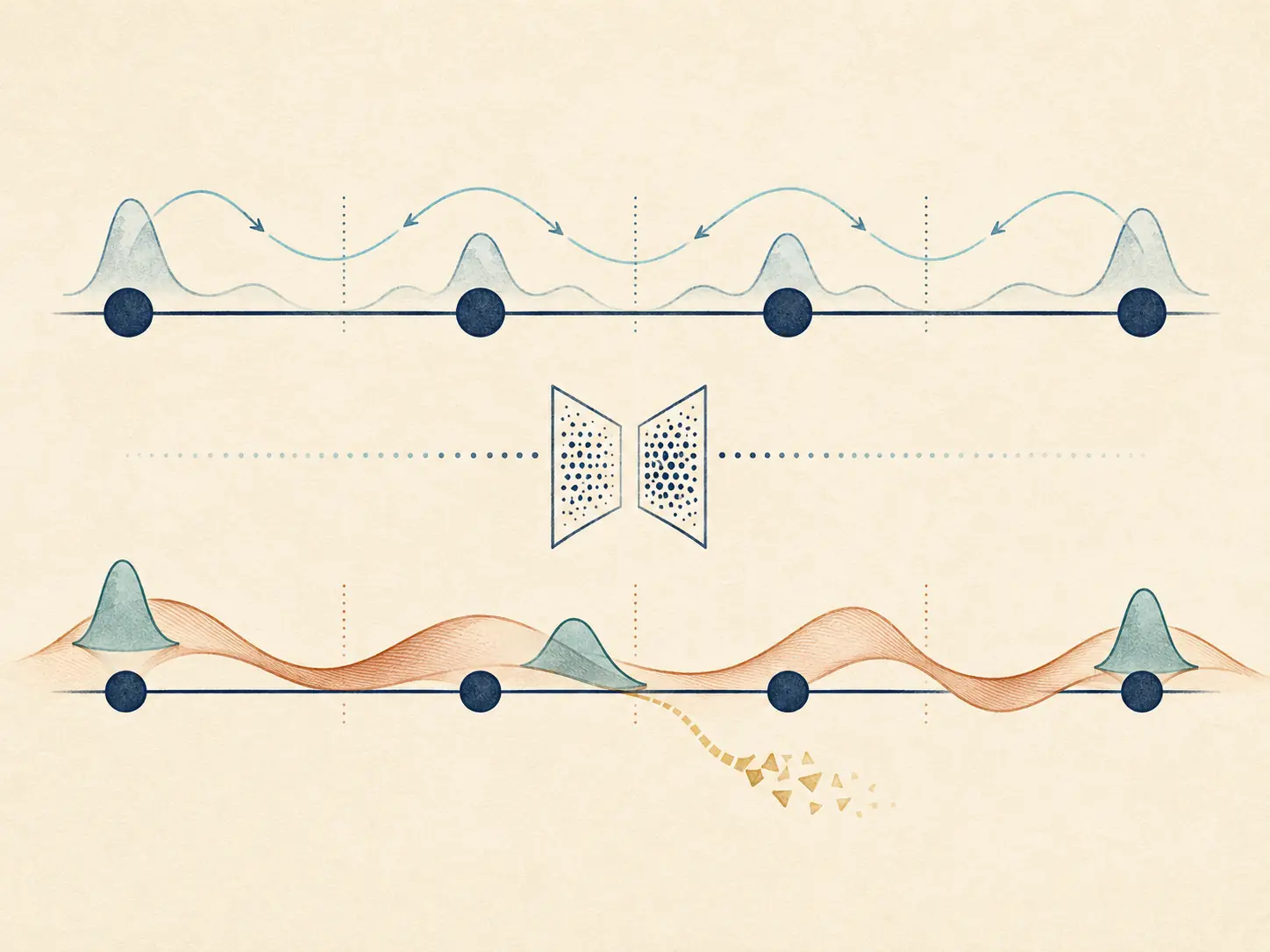
A localized population can change for three different reasons: phases of occupied instantaneous eigenstates can beat; the eigenvectors themselves can change in the fixed localized basis; or a nonadiabatic event can redistribute the magnitudes of the instantaneous-state amplitudes. The paper constructs a target-specific measure that removes the first mechanism while retaining the latter two.

For a fixed target basis state $|X\rangle$, the central question is not simply whether $p_X(t)$ changes, but how much of that change is attributable to following the changing instantaneous eigenstates.

From the paper

Separate phase beating from state following

Write $\widetilde c_k=\widetilde a_k e^{i\widetilde b_k}$ and $d_X^{(k)}=\langle X|\phi_k\rangle$. Differentiating the target population and omitting terms that contain only $\dot{\widetilde b}_k$ defines a real rate $f_X(t)$. Its integral is

When a time-independent Hamiltonian produces large localized-state oscillations, the eigenvectors and coefficient magnitudes remain fixed, so $T_X=0$. In an ideal transfer that follows one changing eigenstate, $T_X$ follows the transferred population. The coefficient-magnitude derivatives must remain in $f_X$ because strongly nonadiabatic events can otherwise create false classifications.

1. ProjectExpress the propagated state in the instantaneous eigenbasis.
2. DifferentiateTrack amplitude magnitudes and fixed-basis eigenvector components.
3. IntegrateAccumulate the non-beating contribution for the chosen target.

From the paper + numerical guidance

A stable numerical workflow

1. Propagate $|\Psi(t)\rangle$ with the desired quantum-dynamics method.
2. Diagonalize $\hat H(t)$ at each saved time.
3. Match neighboring eigenvectors by maximum overlap and align their phases before finite differencing.
4. Evaluate $\widetilde c_k$, $d_X^{(k)}$, their derivatives, and then $f_X(t)$.
5. Integrate $f_X$ and compare $T_X(t)$ with the actual target population.

Simplified educational example

A constant Hamiltonian can transfer population with zero adiabatic contribution

Take $\hat H=\begin{pmatrix}\Delta/2&J\\J&-\Delta/2\end{pmatrix}$ and $|\Psi(0)\rangle=|1\rangle$. For $\Delta=2$ and $J=1$,

import numpy as np
import matplotlib.pyplot as plt

delta, J = 2.0, 1.0
t = np.linspace(0.0, 12.0, 800)
omega = np.sqrt(delta**2 + 4.0*J**2)
p2 = (4.0*J**2/omega**2) * np.sin(0.5*omega*t)**2
T2 = np.zeros_like(t)
plt.plot(t, p2, label="target population")
plt.plot(t, T2, "--", label="adiabatic contribution")
plt.legend(); plt.show()

From the paper

What the measure reveals

In a three-level model it returns zero for transfer generated by constant-coupling beating and follows the target population for counterintuitive, adiabatic coupling pulses. In moving five-molecule aggregates it identifies which part of a mixed adiabatic/nonadiabatic trajectory helped population reach the terminal site. In the paper’s TDDFT-based TCNE trimer example, the reported final ratio is $T_3(t_f)/|c_3(t_f)|^2=0.8$, assigning most but not all of the transfer to adiabatic state following.

Scope and limitations

Where interpretation requires care

• $T_X$ is specific to a chosen target and does not summarize every intermediate transfer.
• An all-state absolute-rate alternative can overcount rapid reversible motion.
• Degeneracies require subspace tracking, and noisy trajectories require careful differentiation.
• The TCNE calculation is a proof of principle with an intentionally fast molecular motion and specific electronic-structure approximations.
• A density-matrix generalization should be derived explicitly rather than assumed from the pure-state formula.